harsha kokel
Model-Agnostic Meta-Learning
My notes on Chelsea Finn, Pieter Abbeel, Sergey Levine, ICML 2017. Written as part of the Complex Networks course by Prof. Feng Chen.
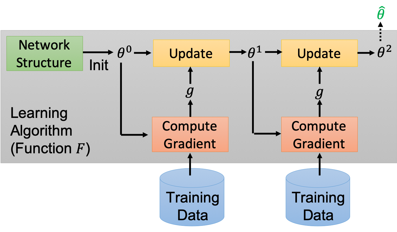
Meta-Learning a.k.a the ‘‘Learning to Learn’’ problem, is the field of study where the researchers are trying to learn the parts of model which in standard machine learning setting are decided by researchers/humans/users. To elaborate, consider for example a standard gradient based machine learning problem. Given a training data and test data, to solve a problem the researches first decide what loss function to optimize and based on existing literature or their expertise they figure out various meta-information of the model. In the figure below, for a standard gradient based machine learning model meta-information like network structure, initialization parameters ($\theta^0$), update method etc are all decided manually.
Meta-learning research aims to learn a model which can help decide such meta-information (all or subset) for any new task.
One of the use-case of meta-learning is in a field called few-shot learning. In few-shot learning, machine learning algorithm is supposed to learn a model for a task from few supervised examples. Meta-Learning can help in few-shot learning by providing a better initialization parameters. Few-shot learning is the problem of learning a model from few examples, meta learning is the problem of learning a model that can easily adapt to the new task from few examples.
This is also the premise of the Model-Agnostic Meta-Learning (MAML) paper by Finn et al 2017.
Transfer-Learning is a research problem in machine learning (ML) that focuses on storing knowledge gained while solving one problem and applying it to a different but related problem1. For Deep Neural Network models, one of the the popular approaches to transfer-learning is by using a pre-trained model. Pre-trained model essentially transfers the knowledge of network parameters between different tasks. This is essentially equivalent to providing initialization parameters for the new task. Transfer-learning via pre-trained model as well as meta-learning use the network parameters of one model as initialization parameters for another model. The difference is in the optimization of the network parameters. While pre-trained model are optimize for some predefined task, meta-learning model are optimized so that they can adapt to new tasks quickly.
The key idea of Model-Agnostic Meta-Learning (MAML) algorithm is to optimize model which can adapt to new task quickly. Consider (pretty similar) tasks ${\mathcal{T}_i , | , i \in { 1,2,3,4}}$ with optimal parameters ${ \theta^{\star}_i , | , i \in {1,2,3,4} }$. Say, for $\mathcal{T}_4$ we have only $k$ supervised examples but we have large number of supervised examples for rest of the tasks i.e. $\mathcal{T}_1, \mathcal{T}_2$ and $\mathcal{T}_3$.
A transfer learning approach will train $3$ different models (with parameters $\theta_1, \theta_2$ and $\theta_3$). Try all three as pretrained model for $\mathcal{T}_4$, compare the performance and pick one that works the best i.e. closest to $\theta_4^{\star}$.
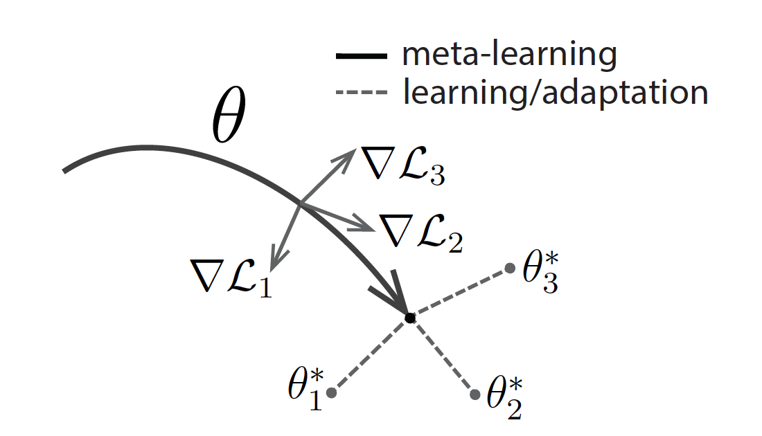
MAML on the other hand uses tasks $\mathcal{T}_1, \mathcal{T}_2$ and $\mathcal{T}_3$ for meta-training and treats them same as task $\mathcal{T}_4$ i.e. only uses $k$ example from each task. MAML learns a single model with parameter $\theta$ in meta-training such that for each task $\mathcal{T}_i$ the gradient step using $k$ examples from that parameter $\theta$ in the direction of $\theta_i^{\star}$ reaches a $\theta^{\prime}_i$. The meta-training objective to bring $\theta^{\prime}_i$ close to $\theta_i^{\star}$. So, the next update of the parameter $\theta$ is a gradient step in a direction calculated as a linear combination of gradient step from $\theta_i^{\prime}$ to $\theta_i^{*}$. This is represented in the figure below, albeit not visibly.
Meta-learning (bold line: —) is performing a search in parameter space such that a gradient step (gray line: →) for any of the training tasks $\mathcal{T}_i, i\in {1,2,3}$ is close to optimal parameters $\theta_i^{\star}$. The parameter $\theta$ is then used as initialization value and fine-tuned for a specific task, this is called learning or adaptation (broken line: - - -).
During meta-training, MAML adapts the parameter $\theta$ for training tasks $\mathcal{T}_i, i\in { 1,2,3}$ to compute the $\theta$ update. In meta-testing, MAML adapts the parameter $\theta$ for test task $\mathcal{T}_4$. We obtain $\theta_4^{\prime}$ by taking gradient step using the $k$ examples.
Parameter $\theta_i^{\prime}$ is computed for any task $\mathcal{T}_i$ using following fine-tuning/learning/adaptation equation.
$$ \theta_{i}^{\prime}=\theta-\alpha \nabla_{\theta} \mathcal{L}_{\mathcal{T}_{i}}\left(f_{\theta}\right) $$
Meta-learning aims to reduce the distance between $\theta_i^{\prime}$ and $\theta_i^{\star}$. Since, $\theta_i^{\star}$ is unknown it instead tries to minimize $\mathcal{L}_{\mathcal{T}_{i}}\left(f_{\theta_{i}^{\prime}}\right)$ for all the tasks. So, meta-objective is:
$$ \min _{\theta} \sum_{\mathcal{T}_{i} \sim p(\mathcal{T})} \mathcal{L}_{\mathcal{T}_{i}}\left(f_{\theta_{i}^{\prime}}\right)=\sum_{\mathcal{T}_{i} \sim p(\mathcal{T})} \mathcal{L}_{\mathcal{T}_{i}}\left(f_{\theta-\alpha \nabla_{\theta} \mathcal{L}_{\mathcal{T}_{i}}\left(f_{\theta}\right)}\right) $$
Note that we restrict our model to minimize the objective of tasks from a distribution $p(\mathcal{T})$.
Meta-optimization is hence done with following update equation:
$$ \theta \leftarrow \theta-\beta \nabla_{\theta} \sum_{\mathcal{T}_{i} \sim p(\mathcal{T})} \mathcal{L}_{\mathcal{T}_{i}}\left(f_{\theta_{i}^{\prime}}\right) $$
Notice that the update equation above depends on the gradient of loss function $\mathcal{L}_{\mathcal{T}_i}\left(f_{\theta_i^{\prime}}\right)$, but $\theta_i^{\prime}$ depends on the gradient of loss function $\mathcal{L}_{\mathcal{T}_{i}}\left(f_{\theta}\right)$. So evidently MAML involves second level gradients.
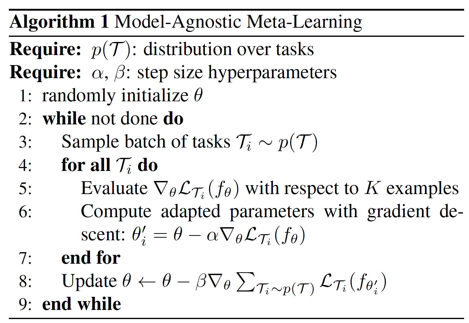
Full algorithm of MAML is quite easy to follow from the above three equations.
Instead of doing the search of $\theta$ for all the tasks in training, like we did in the example above. MAML samples tasks from distribution $p(\mathcal{T})$. In theory, this might just be a distribution of task based on available sample size of each task or distribution based on the similarity to the test task. In practice, they randomly sampled label set from images corpus and then sampled few examples for training and few for testing. To update the parameters $\theta$ in line 8, code computes the second gradient using tensor flow optimizers.
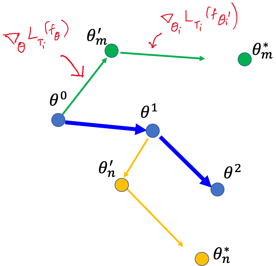
Below figure explains the MAML update equation used in practice. The first arrow for each task is the gradient from fine-tuning equation and the second arrow is from the meta-optimization equation.
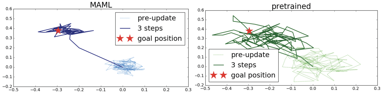
MAML vs Pretrained
The above image highlights the difference between MAML and pretrained models for the MAML-RL in 2D Navigation task. While the MAML model can adapt to the new task quickly, the pre-trained models take longer.
First-order MAML
Since the MAML involves second-order derivative, it can be computationally expensive. Authors propose a first-order approximation for such scenarios, by omitting the second order derivatives.
Since,
$$ \nabla_{\theta} \sum_{\mathcal{T}_{i} \sim p(\mathcal{T})} \mathcal{L}_{\mathcal{T}_{i}}\left(f_{\theta_{i}^{\prime}}\right) = \sum_{\mathcal{T}_{i} \sim p(\mathcal{T})} \nabla_{\theta} \mathcal{L}_{\mathcal{T}_{i}}\left(f_{\theta_{i}^{\prime}}\right) \\ = \sum_{\mathcal{T}_{i} \sim p(\mathcal{T})} \nabla_{\theta_i^{\prime}} \mathcal{L}_{\mathcal{T}_{i}}\left(f_{\theta_{i}^{\prime}}\right) \cdot \nabla_{\theta} (\theta_i^{\prime}) $$
In first-order MAML, authors use $\nabla_{\theta} (\theta_i^{\prime}) \approx 1$
Reptile
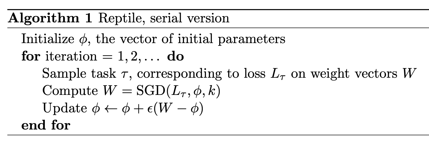
Reptile further simplifies the gradient computation of MAML by proposing following algorithm.
Notice that the initial parameter $\theta$ used in MAML is equivalent to $\phi$ in the reptile algorithm.
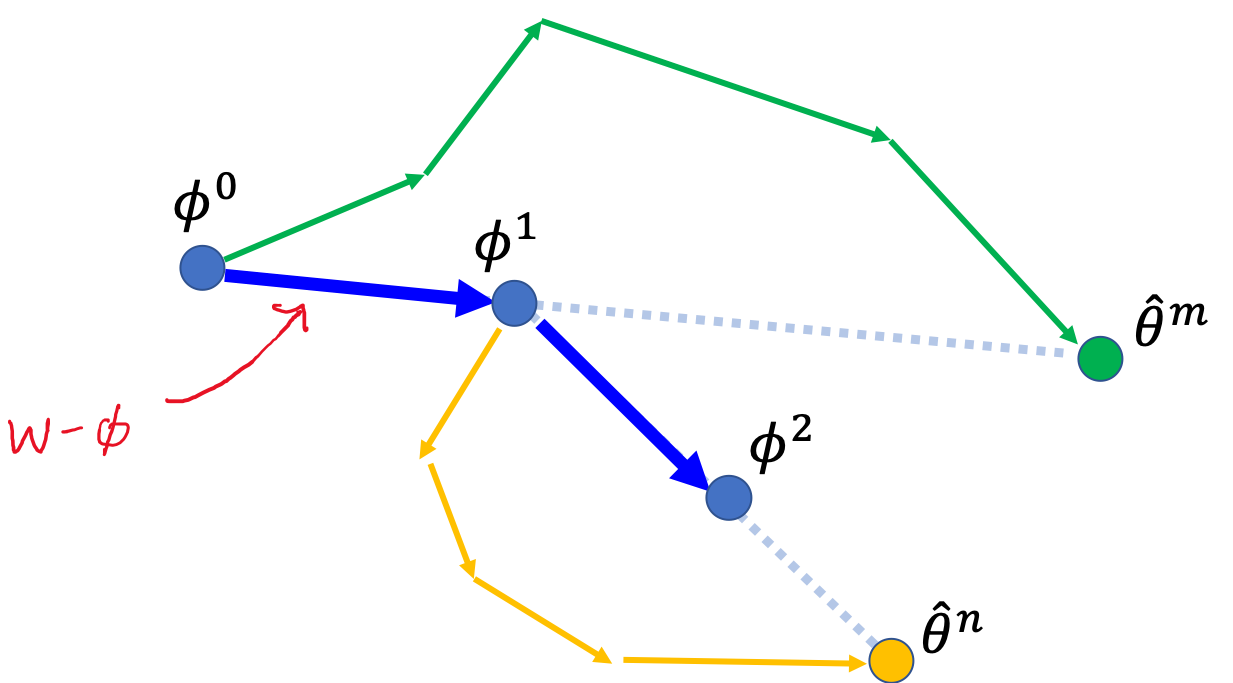
Instead of computing the $\theta^{\prime}_i$ for each task with one step gradient, Reptile computes parameter $W$ by running stochastic gradient descent for $k$ steps. Then instead of computing the gradient w.r.t the task for updating the initial parameter $\theta$ (as done in line 8 of MAML), Reptile recommend to just shift the initial parameter in the direction of $W$ by using $(W - \phi)$ as gradient. Below figure explains the Reptile update process.
References
- Definition of transfer learning from Wikipedia
- ICML 2019 Meta leraning tutorial
- Prof. Hung-yi Lee’s slides on meta learning
- Reptile paper: Alex Nichol, Joshua Achiam, John Schulman On First-Order Meta-Learning Algorithms, 2018
- Reptile Blog
- Code: Deep Metalearning using “MAML” and “Reptile”