harsha kokel
Tools for Causal Inference
I read the Book of Why last year and recently in the reading group at Starling lab we read the 7 Tools of causal inference by Prof. Pearl. I was a little taken by how much I have forgotten about causal inference. So I found the need to jolt down my understanding, so I can refer to it later. This article summarized my current understanding of the tools presented in the paper, based on the paper and the book.
There is enough motivation now showing the necessity of learning models that have a correct causal structure. The famous “Correlation is not causation” quote should ring a bell. Although the research on learning causal structure from observed data has not yet shown its potential. There are certain tasks from causal literature which can still be solved by just using observed data. Specifically, interventional and counterfactual queries can still be answered if we know the causal structure. And, to do that we need the following tools of causal inference popularized by Prof. Pearl.
Tool 1. Encoding causal assumptions: Transparency and testability.
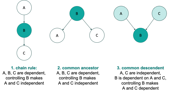
Tool 1 emphasize the importance of graphical representation of causality using a Bayesian Network. By representing the causal influences using BN, we can leverage the three rules of conditional independences for inference.
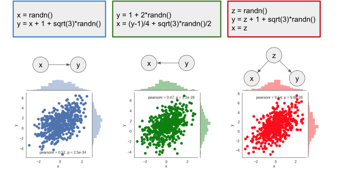
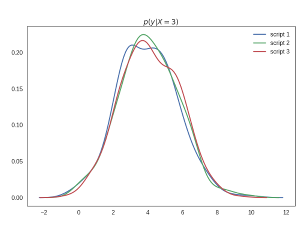
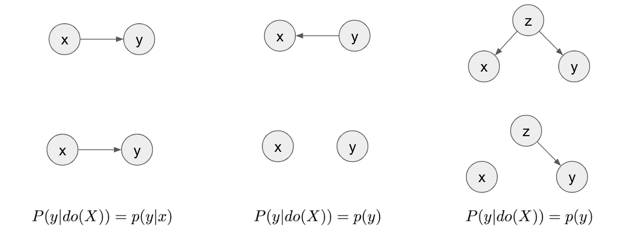
Although very powerful, the BN representation is limited. Only with graphical representation we will not be able to differentiate between $P(y|X=3)$ and $P(y|do(X=3))$. Ferenc Huszár gives a beautiful explanation of the difference between the two in his post on causal inference 1. Given different causal BN and data generated from different distributions as shown in the figure below, we can see that the joint distribution of $x$ any $y$ is identical. Even the conditional probability $P(y|X=3)$ is identical.
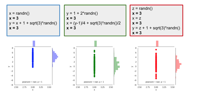
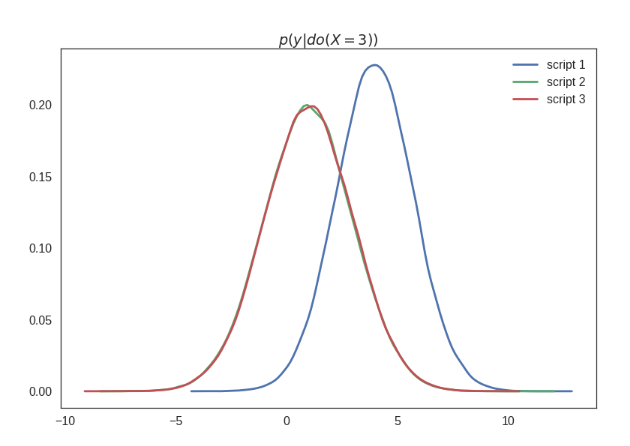
But, what if we force the variable $x$ to take a fixed value $3$ in each of these cases, i.e. intervene on variable $x$? Should we still expect the distribution of y to be same? No. As expected the impact of intervening on variable $x$ has different impact on values of $y$. This is evident in the two distribution plotted below.
Above values of $p(y|do(X=3))$ is computed by generating the data after forcing $x=3$. In machine learning, we want to learn the impact of assigning value $x=3$ without re-generating the data. So, how do we compute $p(y|do(X=3))$ without generating the data? We need more advanced tools for that.
Tool 2. Do-calculus and the control of confounding.
In the above example, intervening on variable $x$ and fixing it to $3$ is like making $x$ independent of all its ancestor. So, we remove all the incoming edges to $X$. Now, Computing $P(y|X=3)$ of the resulting graph will give us $P(y|do(X=3))$ of the original graph.
This is what do-calculus is. The process of mapping the do-expressions to the standard conditional probability equations using the three rules. The probability equations we get at the end are called estimand and the the value obtained after computing the estimand on the observed data is called estimate.
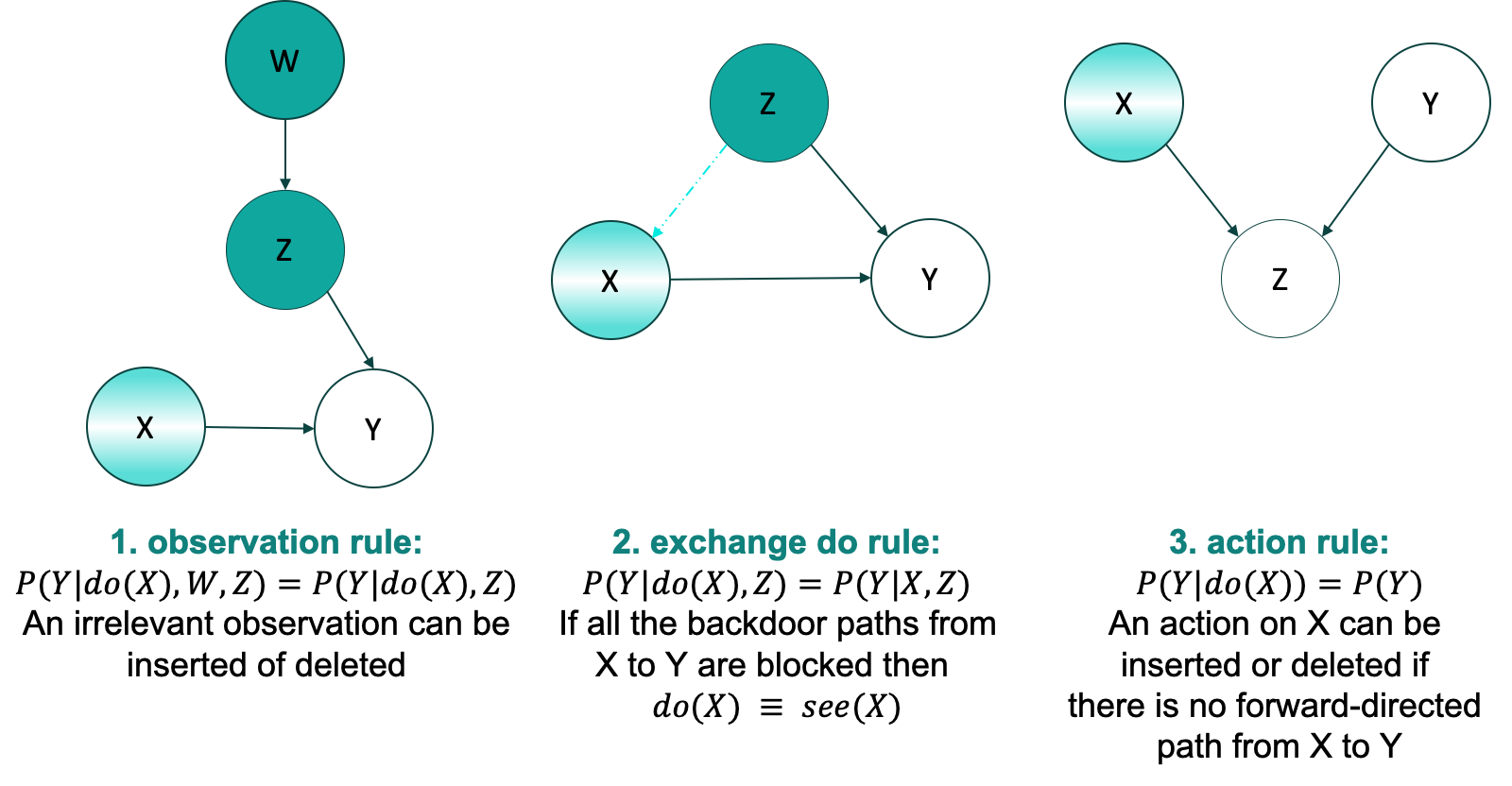
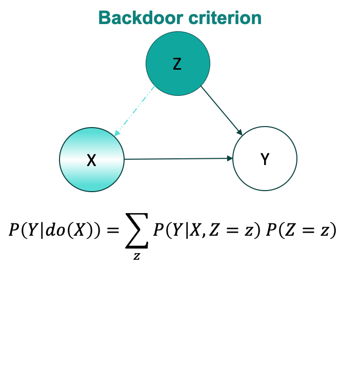
One of the most common adjustment in the causal inference is de-confounding i.e. adjusting for all the common causes (confounders) of two variables. This is the famous backdoor criterion. Back-door path for $X \rightarrow Y$ is any path that ends in $Y$ and has arrow pointing into $X$. To de-confound $X$ and $Y$, we have to block all the back-door path by adjusting for (i.e. conditioning on) variables which either follow chain-rule or common ancestor rule. We have to be very careful to not condition on any common descendent in the back-door path.
For graphs where we are unable to block the back-door path (say, because of unobservable variable), do-calculus gives us a work-around. This is commonly called the front-door criterion.
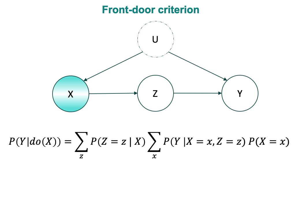
For graph given above, the front-door formula is derived as follows:
$$ \begin{aligned} P(Y |do(X= \tilde{x})) & = \sum_z P(Y|do(X = \tilde{x}), Z=z) P(Z=z|do(X = \tilde{x})) \\ & \quad \quad \quad \quad \quad \quad \quad \quad \quad \quad \quad \quad \rhd \text{probability axiom} \\ & = \sum_z P(Y|do(X= \tilde{x}),do(Z=z)) P(Z=z|do(X= \tilde{x})) \\ & \quad \quad \quad \quad \quad \rhd \text{ back door-path between X and Y is blocked by X,} \\ & \quad \quad \quad \quad \quad \quad \quad \quad \text{so we apply exchange do-rule } \\ & = \sum_z P(Y|do(X= \tilde{x}),do(Z=z)) P(Z=z|X= \tilde{x}) \\ & \quad \quad \quad \quad \quad \rhd \text{exchange do-rule, back door-path between X and Z } \\ & \quad \quad \quad \quad \quad \quad \quad \quad \text{ is blocked by common descendent Y} \\ & = \sum_z P(Y|do(Z=z)) P(Z=z|X= \tilde{x}) \\ & \quad \quad \quad \quad \quad \rhd \text{action rule, No forward path from X to Y } \\ & \quad \quad \quad \quad \quad \quad \quad \quad \text{ as do(Z) blocks it.} \\ & = \sum_z \left( \sum_x P(Y|X=x, Z=z) P(X=x) \right) P(Z=z|X= \tilde{x}) \\ & \quad \quad \quad \quad \quad \quad \quad \quad \quad \quad \quad \quad \quad \rhd \text{using back-door adjustment } \\ & = \sum_z P(Z=z|X= \tilde{x}) \sum_x P(Y|X=x, Z=z) P(X=x) \\ & \quad \quad \quad \quad \quad \quad \quad \quad \quad \quad \quad \quad \quad \rhd \text{same as front-door criterion } \\ \end{aligned} $$
Its amazing, to compute the $P(Y | do(X= \tilde{x}))$, we have to sum over all the possible assignments of $x$. With only Tool 1, I would have mostly computed probability by only looking at data points where $X = \tilde{x}$.
Tool 3. The algorithmitization of counterfactuals.
Thumb rule of counterfactual
counterfactuals talks about a specific individual/event/scenario.
Counterfactual queries are questions about a parallel universe where one(or few) feature(s) is(are) different for a specific example, not on the whole population. It is a question always asked in retrospection for a specific instance. For example, An interventional question to analyze importance of wearing mask during current pandemic can be asked as “What would be the total number of COVID-19 positive patients, if we banned mask in public?” i.e $P($ COVID_Pos $| , do($ wear_mask $= 0) )$. But a counterfactual question would be “Given that I had worn mask when I went to buy grocery last week and I do not have COVID-19 today, what would have happened if I had not worn mask?” This question is about me, and about a specific instance of not wearing mask. This counterfactual question has to account for every variable which is not a descendent of wear_mask staying exactly the same. So, the fact that I drove to the TomThumb or the cart which I used should stay the same, because in my assumed causal graph, they are not descendants of wear_mask variable. But on the other hand the fact that I washed my hands and face for exactly 12 secs after coming home, and that I entered the spice aisle might change. Because in my causal assumption these are descendent of wearing mask. Hey! I would have washed hands and face for 20 secs if I was not wearing mask and I would have definitely not entered the spice aisle which had like 3 people in there. I would have maintained six feet distance.
So, mathematically the counterfactual query is $P(h_c^*=1|h_m^\ast=0,h_c=0, h_m=1,..)$, where, $h_c$ is Harsha has COVID-19, $h_m$ is Harsha wore mask, and \ast indicates counterfactual universe. So, all the variable that are not descendants of $h_m$ will stay same i.e $h_i = h_i^\ast, \forall i \notin Des(h_m)$. To compute the probability of the counterfactual query, we need more than the do-calculus from Tool-2. We need structural equation models (SEMs) and an algorithm.
I strongly recommend Ferenc Huszár’s post on counterfactuals for more clarity on how the interventional probability $P(Y| do(X))$ is the computation on population, but counterfactuals is for individuals.
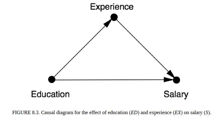
Let’s see how we use tool 3 to answer the counterfactual query, “What would Alice’s salary be if she had a college degree?”. This query is from the fictitious employee data reproduced below from The Book of Why. Here, the experience is mentioned in number of years and three levels of education are : 0 = high school degree, 1 = college degree, 2 = graduate degree. The assumed causal graph is also shown below.
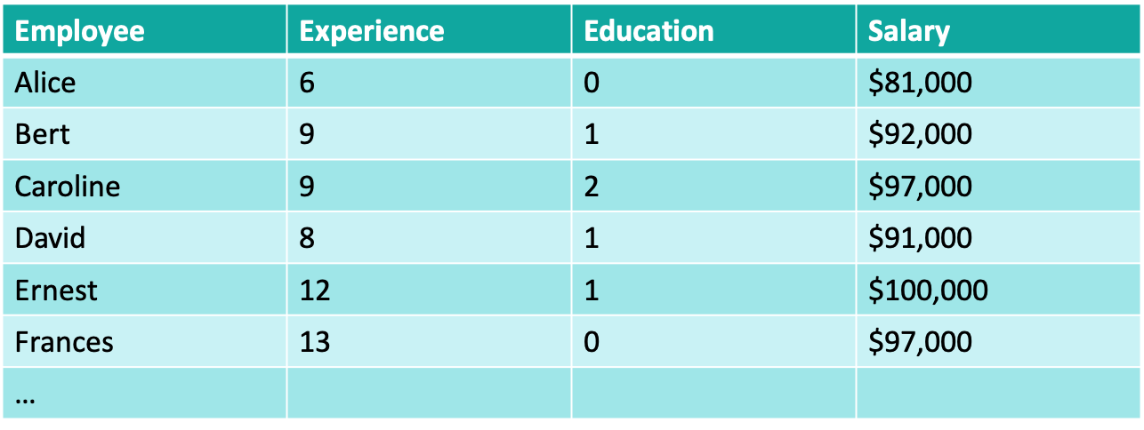
src: The Book of Why
The SEM for this graph will be:
$$ f_0(Ed) = , U_{0} \\ f_1(Ex) = b_1 , + , a_1 Ed , + , U_{1} \\ f_2(S) = b_2 , + , a_2 Ed , + a_2 Ex , + , U_{2} $$
Here, U are unobserved idiosyncratic variables which capture the peculiarity of the individual in question. So, these values are different for each user. For instance, We can think of $U_2$ accounting for difference in salary as some artifact of individuals unobserved characteristics which is independent of level of education and experience (say, time management). In terms of graphical model, we can think of these variables as parents of the variable on the left side of the equation. Note that these idiosyncratic variables do not have incoming arrows. So, given the counterfactual explanation above, these values should remain unchanged in the parallel universe. If we were to do linear regression we would have an $\varepsilon$ instead of $U$ to adjust for the noise. However, the noise is then a random parameter which is not necessarily kept constant across universe. This is where the SEM differ from linear regression.
The SEM coefficients can be estimated from the observed data, much like linear regression.
$$ f_1(Ex) = 10 – 4 Ed + U_1 \\ f_2(S) = 65,000 + 5,000 Ed + 2,500 Ex + U_2 $$
Now, the algorithm to compute the counterfactual query is these three steps:
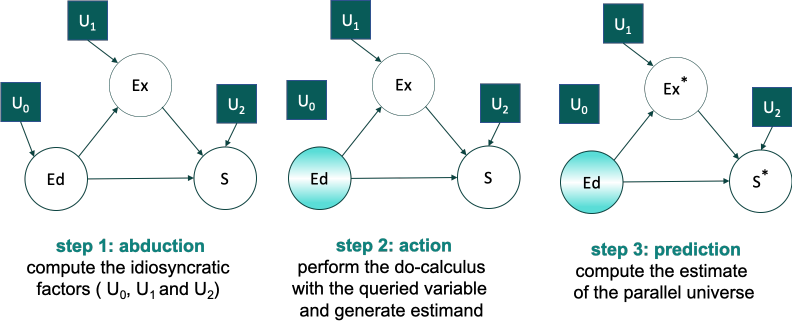
Following these steps for Alice here, in step 1 we find that $U_1(Alice) = , –4$ and $U_2(Alice) = $1,000$. We do not actually care for $U_0(Alice)$ because in step 2 we set $f_0(Ed(Alice)) = 1$. 1 for college degree, and remove all incoming arrows to $Ed$ and perform do-calculus adjustments. Here, since there are no causal parents of $Ed$, our SEM model equations $f_1$ and $f_2$ do not change. Then, in step 3, we estimate the counterfactual parameters, $Ex^\ast(Alice) = 2$ and $Ed^\ast(Alice) = 76000$.
Rest of the tools…. to be added later.
Critique
I certainly believe that the advent of ML and AI necessitates the task of learning the causal structure from observed data. The three tools mentioned above do not do that. They assume the causal structure is provided. These tools provide us the correct way of utilizing the causal structure in machine learning. I believe most of the machine learning models build for classification/regression tasks assume some form of causal structure already. What is not clear is, if those models correctly leverage the causal structure that they are assuming. These tools help us answer that. The question about whether or not the causal structure assumed is correct or not can be subjective and task specific. The three tools mentioned above certainly do not answer that.
References
- The Book of Why: The New Science of Cause and Effect by Judea Pearl and Dana Mackenzie
- The Seven Tools of Causal Inference, with Reflections on Machine Learning by Judea Pearl
- 1https://www.inference.vc/causal-inference-2-illustrating-interventions-in-a-toy-example/
- Causality: Models, Reasoning and Inference by Judea Pearl