harsha kokel
Understanding Attention and Generalization in Graph Neural Networks
My notes on Boris Knyazev, Graham W. Taylor, and Mohamed R. Amer, NeurIPS 2019. Written as part of the Complex Networks course by Prof. Feng Chen.
Attention in CNNs
Attention in CNNs is reweighting the feature map $X \in \mathbb{R}^{N \times C}$, to provide attention to some nodes.
$$ \begin{aligned} Z & =\alpha \odot X \quad (Z_{i}=\alpha_{i} X_{i}) \\ \text{such that,} \quad \quad & \sum_{i}^{N} \alpha_{i} = 1 \\ \odot & \text{ is element-wise multiplication} \end{aligned} $$
Note: $\alpha_i$ is a scalar and $X_i$ is vector of size C. So, $Z_i$ is also a vector of size C. $Z \in \mathbb{R}^{N \times C}$
Pooling in CNNs
Pooling in CNNs divide the grid into local regions uniformly (not neighbors) and aggregate them to reduce the dimension.
src: stackoverflow
So, there is no parallelism between attention and pooling in the CCNs.
But in GNN, pooling also use the neighborhoods.
Top K Pooling
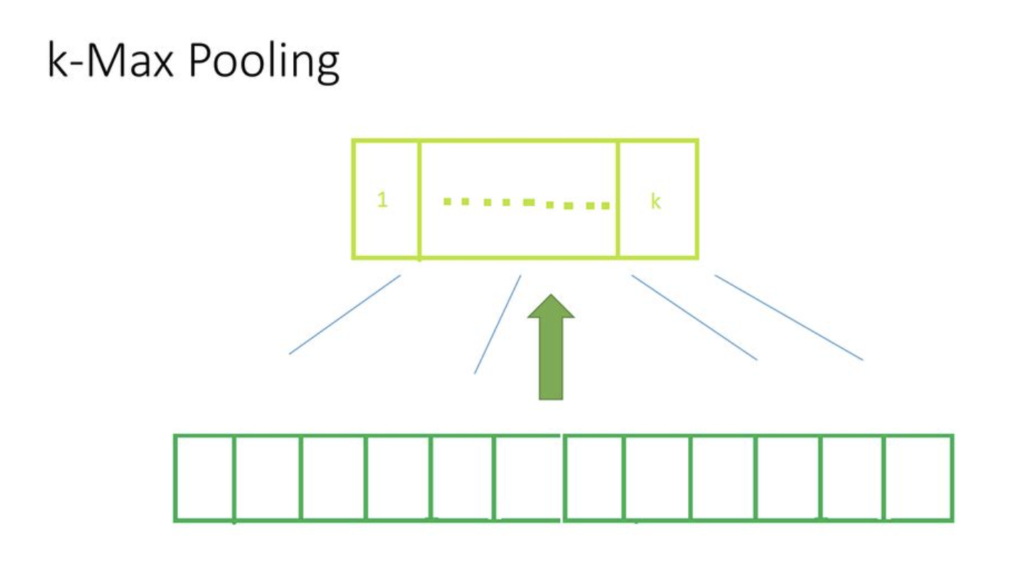
Top K pooling was proposed by Gao and Ji, Graph U-Nets, ICML 2018, it is supposed to be a equivalent of k-max pooling (generalization of max-pooling) in the CNN where each feature map is reduced to size k by picking units with highest values. Since, in GNN the k-highest values can possibly come from different node for each feature-map the straight forward extention of k-max pooling does not work. So, Gao and Ji propose to project all the nodes to 1D and then select top K from that.
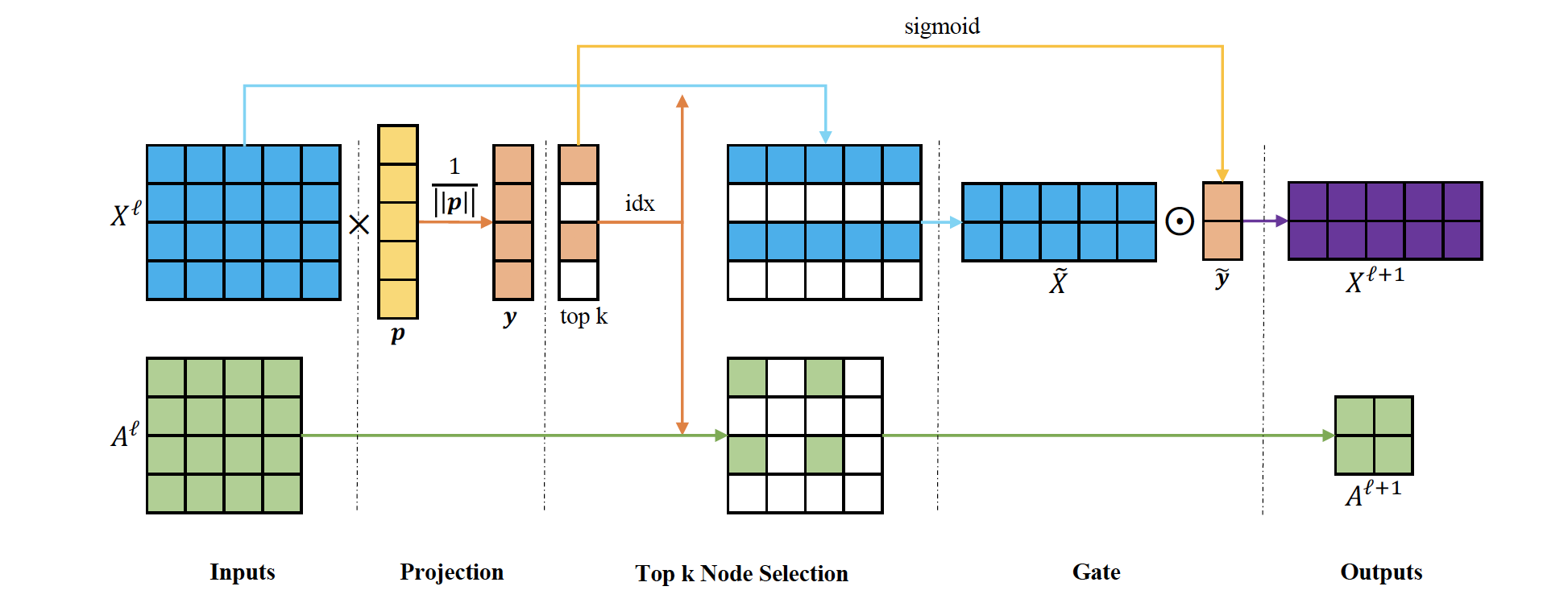
Given feature matrix $X^{\ell} \in \mathbb{R}^{N \times C}$ and adjacency matrix $A^{\ell} \in \mathbb{R}^{N \times N}$, first project the feature matrix to 1D using projection vector $\mathbf{p}$ and normalize it,
$$ \mathbf{y}=\frac{X^{\ell} \mathbf{p}^{\ell}}{\left|\mathbf{p}^{\ell}\right|} $$
From this normalized 1D representation of each node ($\mathbf{y}$), filter top K nodes and use indexes ( $\mathrm{idx}=\operatorname{rank}(\mathbf{y}, k)$) to retrieve relevant feature matrix and adjacency matrix.
$$ \begin{aligned} \tilde{X}^{\ell} &=X^{\ell}(\text { idx}, :) \\A^{\ell+1} &=A^{\ell}(\mathrm{idx}, \mathrm{idx}) \end{aligned} $$
However, since the $\mathbf{y}$ is discrete valued, authors use gate operation ($\operatorname{sigmoid}$) to convert $\mathbf{y}$ to real value and make it eligible for back-propagation $(\tilde{\mathbf{y}} = \operatorname{sigmoid}(\mathbf{y}(\mathrm{idx}))$. The final feature matrix for the next layer is obtained by element wise multiplication of feature vectors of selected nodes and $\tilde{\mathbf{y}}$,
Over all,
$$ \begin{aligned} X^{\ell+1} & =\tilde{X}^{\ell} \odot\left( \tilde{\mathbf{y}}\mathbf{1}_{C}^{T}\right) \\ \text{with} \quad \tilde{\mathbf{y}} & = \operatorname{sigmoid}(\frac{X^{\ell} \mathbf{p}^{\ell}}{\left|\mathbf{p}^{\ell}\right|}(\mathrm{idx})) \end{aligned} $$
In GNNs, there is a parallelism between pooling and attention. Node attention $\alpha$ can be thought of as $\mathbf{\tilde{y}}$.
$$ Z_{i}=\left\{\begin{array}{ll}{\alpha_{i} X_{i},} & {\forall i \in P} \\{\emptyset,} & {\text { otherwise }}\end{array}\right. $$
where, $P = \{\text{idx}\}$ and $|P| = k$. $P$ is obtained by finding the indices of top-k values of $\mathbf{y}$, which is computed by learning projection vector $\mathbf{p}$ using back-propagation on input graph.
This paper proposes to combine the attention and pooling to a single computational block, which does not have a fixed $k$. Instead, set $P$ is determined by threshold $\tilde{\alpha}$:
$$ Z_{i}=\left\{\begin{array}{ll}\alpha_{i} X_{i}, & \forall i: \alpha_{i}>\tilde{\alpha} \\\emptyset, & \text { otherwise }\end{array}\right. $$
Further, they also propose a combination of GIN and ChebyNet called ChebyGIN to be used for convolution after pooling.
ChebyGIN
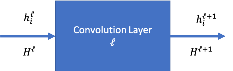
Graph Convolutional Network (GCN), Graph Isomorphism Network (GIN), ChebyNet have similar formulation with minor changes. The proposed ChebyGIN formulation is an extention of these changes. This section highlights the equivalence and differences in the mathematical forms of these networks. We compare the Convolution layer of these networks, each take input $H^{(\ell)}$ (equivalently $h_i^{(\ell)}, \forall i \in V$) and outputs $H^{{\ell+1}}$ (equivalently $h_i^{(\ell+1)}$). And, $\mathcal{N}(i)$ indicates neighborhood of the node $i$.
GCN:
$$ \begin{aligned} H^{(\ell+1)} &= \sigma\left(\hat{A} H^{(\ell)}\mathbf{W}^{(\ell)}\right) \\ \mathbf{h}_{i}^{(\ell+1)} & = \sigma\left( \frac{1}{\mathcal{c}_{ii}} \mathbf{h}_{i}^{(\ell)} \mathbf{W}^{(\ell)} + \sum_{j \in \mathcal{N}(i)} \frac{1}{\mathcal{c}_{ij}} \mathbf{h}_{j}^{(\ell)} \mathbf{W}^{(\ell)}\right) \\ \text{with, } c_{ij} = \sqrt{d_i, d_j} & \text{ and } d_i = |\mathcal{N}(i)| \end{aligned} $$
GIN:
Replaces $\sigma$ with multi-layer perceptron (MLP) and since, the MLP has weights and does rescaling from $f^i$ to $f^o$, we do not need $\mathbf{W}^{(\ell)}$ and the normalization $(\frac{1}{\mathcal{c}_{ij}})$.
$$ \mathbf{h}_{i}^{(\ell+1)} = \operatorname{MLP}\left( \mathbf{h}_{i}^{(\ell)}(1 + \varepsilon^{(\ell)}) + \sum_{j \in \mathcal{N}(i)} \mathbf{h}_{j}^{(\ell)}\right) $$
Here, when $\varepsilon > 0$ the current node is given more importance, when $\varepsilon = 0$ the current node has same importance.
ChebyNet:
Generalization of GCN to $k^{th}$ order approximation of Chebyshev polynomial.
$$ \mathbf{h}_{i}^{(\ell+1)} = \sigma\left( \sum_{k =1}^{K-1} \left( \left( \frac{1}{\mathcal{c}_{ii}^{k}} \mathbf{h}_{i}^{(\ell)} \mathbf{W}^{(\ell)} \right) + \theta_k \sum_{j \in \mathcal{N}_{k}(i)} \frac{1}{\mathcal{c}_{ij}^{k}} \mathbf{h}_{j}^{(\ell)} \mathbf{W}^{(\ell)}\right) \right) $$
ChebyGIN:
Replaces $\sigma$, $\mathbf{W}$ and $\frac{1}{\mathcal{c}_{ij}^{k}}$ of ChebyNet, same as GCN.
$$ \mathbf{h}_{i}^{(\ell+1)} = \underbrace{\operatorname{MLP}}_{\text{FC Layer}}\left( \underbrace{ \sum_{k =1}^{K-1} \mathbf{h}_{i}^{(\ell)}d_i(1 + \varepsilon^{(\ell)}) + \theta_k \sum_{j \in \mathcal{N}_{k}(i)} \mathbf{h}_{j}^{(\ell)} d_j}_{\text{GNN Layer}} \right) $$
$\theta_k$ is still multiplied at the neighborhood level to obtain different weights for each neighborhood. All the node feature vectors ($h_i$) are multiplied by node degree ($d_i$) for first layer.
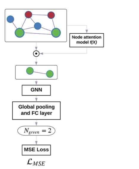
Proposed architecture
The proposed architecture is as follows: first layer is a attention/pooling of input graph, second layer is GNN which aggregates features from local neighborhoods, and third layer is a fully connected (FC) layer, which can also do global pooling and finally an output layer which will be used for training. A separate fully connected MLP called attention network is trained to obtain attention values on each node.
Attention Network
For supervised learning of the attention network, the ground truth of attention values for each node ($\alpha_i^{GT} \in [0,1]$) in the graph is obtained by heuristic.
For example, in experimental dataset for graph color count, attention on each node is defined as follows:
$$ \alpha_{i}^{GT}=\left\{\begin{array}{ll}{\frac{1}{|N_{green}|},} & {\forall i \in N_{green}} \\{0,} & {\text { otherwise }}\end{array}\right. $$
In experimental dataset of graph triangle count, following heuristic is used;
$$ \alpha_{i}^{GT}=\left\{\begin{array}{ll}{\frac{T_{i} }{\sum_{i} T_{i}},} & {\forall i \in \text{Triangle } } \\ {0,} & {\text { otherwise }}\end{array}\right. \\ \text{with, } T_i = \text{number of triangles that include node } i $$
For MNIST-$75SP$ dataset where each node is a superpixel and edges are formed based on spatial distance between superpixel centers, following heuristic was used:
$$ \alpha_{i}^{GT}=\left\{\begin{array}{ll}{\frac{1}{N_{nonzero}},} & {\forall i \in \text{Nonzero intensity superpixel} }\\ {0,} & {\text { otherwise }}\end{array}\right. \\ \text{with, } N_{nonzero} = \text{number of such pixels } i $$
Training
These networks are trained using back-propagation to minimize the Mean-Squared Error (MSE) loss or the Cross-Entropy loss (CE) of the over all prediction and minimize the Kullback-Leibler (KL) divergence loss between ground truth attention $\alpha^{GT}$ and predicted coefficients $\alpha$. The KL term is weighted by scale $\beta$ and number of nodes $N$.
$$ \mathcal{L}=\mathcal{L}_{M S E / C E}+\frac{\beta}{N} \sum_{i} \alpha_{i}^{G T} \log \left(\frac{\alpha_{i}^{G T}}{\alpha_{i}}\right) $$
Since $\sum_i \alpha_i = 0$, $\alpha$ can be thought of as a probability distribution of attention over all the nodes and so, minimizing the KL-divergence is an obvious first choice. Below equation shows relationship between cross-entropy, entropy and KL Divergence. (Answer Q-5)
$$ H(p, q)=H(p)+D_{\mathrm{KL}}(p | q) $$
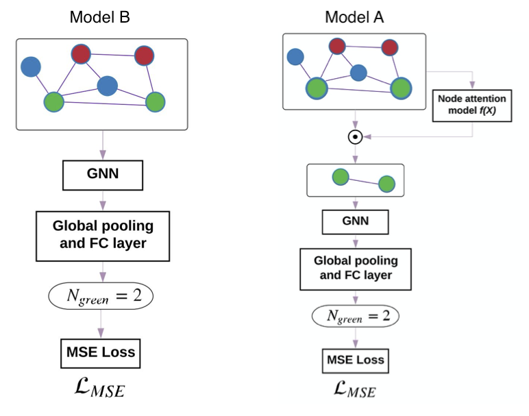
Weakly supervised model
For domains where the ground truth of attention is hard to obtain for each node, authors propose a weakly supervised learning setting as follows. Train an attention network (model B), which has same structure as the proposed architecture (model A) except for attention/pooling layer. Model B is trained to reduce the $\mathcal{L}_{MSE}$ for $y$ prediction. Then, the $\alpha^{WS}$ is calculated using the trained model and input graph $G$.
$$ \begin{aligned} {\alpha}_{i}^{W S} & =\frac{\left|y_{i}-y\right|}{\sum_{j=1}^{N}\left|y_{j}-y\right|} \\ \text{with } y & = \operatorname{ModelB}(G) \\ \text{ and } y_i & = \operatorname{ModelB}(G - \{N_i\}) \\ \end{aligned} $$
Next, the proposed architecture – Model A is trained using $\alpha^{WS}$ to optimize both the MSE and KL divergence.
For colors domain, authors use 2 layers of GNN. So mathematical form for model B is:
$$ Y = \operatorname{GNN}(\underbrace{W^{1}}_{64 \times 1},\operatorname{GNN}(\underbrace{W^{0}}_{64 \times F^i}, \underbrace{H}_{N \times F^{i}} ) ) $$ where as mathematical form of model A is:
$$ Y = \operatorname{ChebyGIN}(\underbrace{W^{1}}_{64 \times 1},\operatorname{ChebyGIN}(\underbrace{W^{0}}_{64 \times F^i}, \alpha^{WS}X) ) $$
where $\alpha^{WS}$ is as defined above, obtained from model B.
Analysis
How powerful is attention over nodes in GNNs?
Contrary to what the authors mention in the paper, I feel that the experimental results show that there is not a lot of co-relation between attention and model accuracy. The example result below shows that the even though the proposed model has high co-relation with attention AUC, there are other models which do not show better performance even when the attention AUC is high. This observation is also backed by the paper, Jain et al. NAACL 2019 Attention is not Explanation.
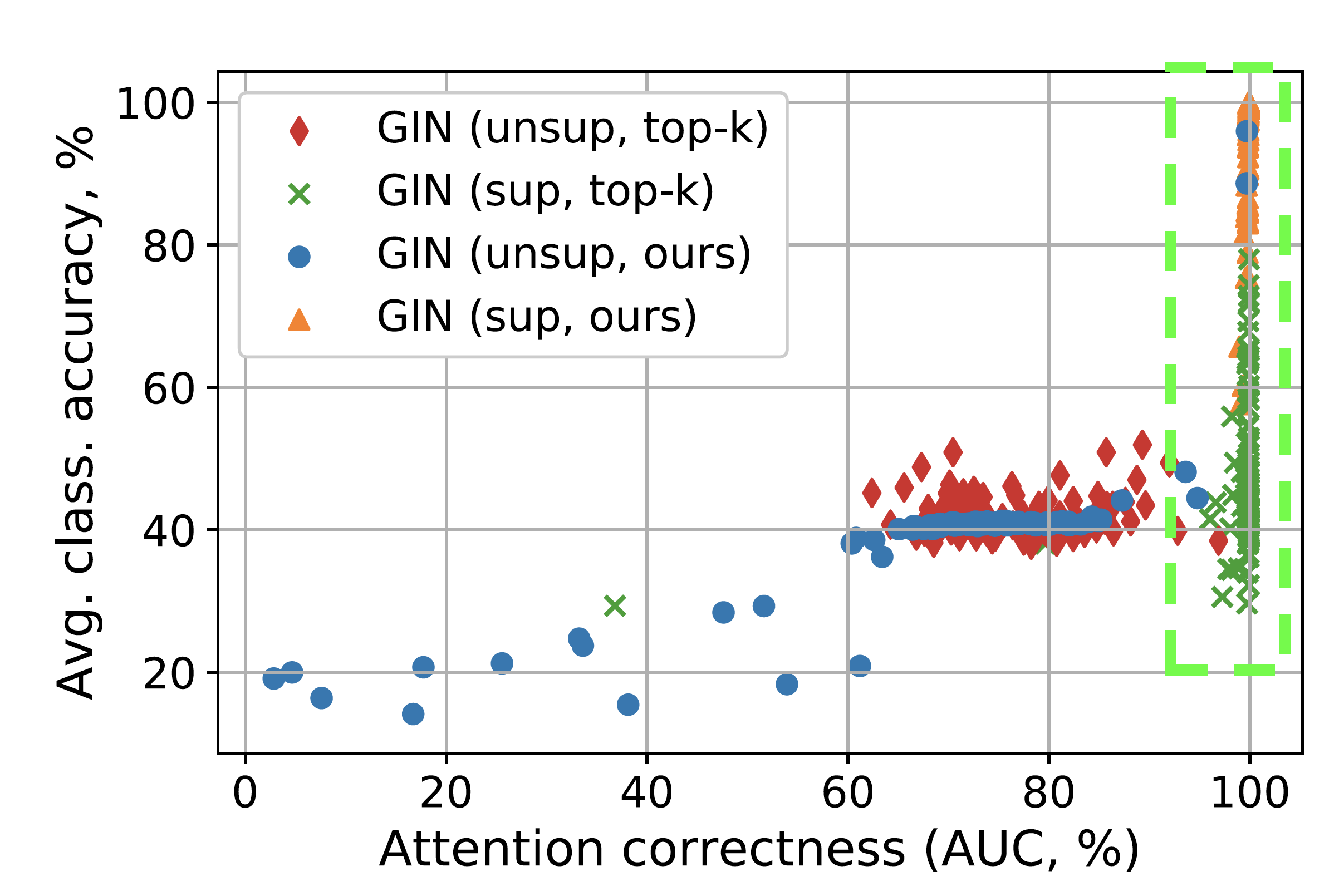
src:Knyazev et. al 2019 [Fig 3a]
So the power of attention over nodes is I think need more study.
What are the factors influencing performance of GNNs with attention?
From experiment results it seems following factors influence the GNNs with attention:
- initialization vector – optimal initialization has better accuracy in Fig-4(c)
- quality of the attention – Supervised attention has better results than weakly supervised attention.
- strength of GNN model used – ChebyGIN model has better results than GIN/GCN
Why is the variance of some results so high?
Variance of some results is high because the model is very sensitive to the initialization parameters. It is only able to recover from bad initialization of hyper-parameters when the attention is good. Bad initialization of attention was not recoverable.
How top-k compares to our threshold-based pooling method?
Experiments show that threshold-based pooling has better results than top-k pooling for larger datasets (with high features).
How results change with increase of attention model input dimensionality or capacity?
With increase in the input dimension for the attention model, the distribution of $\alpha$ values become flat ($\because \sum_i\alpha_i = 1$). Experiments show that in such cases, deeper GNN model for attention are useful.
Can we improve initialization of attention?
Authors observe for unsupervised attention models, normal or uniform distribution with high values is preferred for the initialization of parameters of attention model. But for supervised or weakly supervised model smaller values are preferred. There is no intuition on why one is preferred over the other, paper just states the observation based on empirical evaluations.
What is the recipe for more powerful attention GNNs?
Recipe for powerful attention is to get supervision for attention. If supervision is not possible, use the weakly-supervised method for attention.
How results differ depending on to which layer we apply the attention model?
Although it is desirable to use attention model closer to the input layer to reduce graph size and keep the attention weights interpretable, the experiments show that the attention on deeper layer have higher impact on the performance.
Why is initialization of attention important?
Since the final model is trained by considering the $\alpha$ – attention weights as final, when the attention those weights have bad initialization, the weights learnt in rest of the model are wrong and hence the model is not able to recover.
However, I feel that the models should be able to recover from the bad initialization with more iterations. Literature of expectation-maximization and bi-level optimization indicates that this is possible.
Doubts
- Why use sigmoid in Top-K Pooling? Gate operation – why is projection discrete ??
Questions
- What is the dimensionality of $Z_{i}$ ? Link to Answer
- How to decide $P$ from input graph? Link to Answer
- Provide mathematical form of ChebyGIN and show all the parameters Link to Answer
- Why is $KL$ selected as the loss function, but not cross entropy and squared error? Link to Answer
- Relation between Cross entropy and KL Divergence. Link to Answer
- Give mathematical forms of model A and B for Colors. Link to Answer
- Summarize: How powerful is attention over nodes in GNNs? Link to Answer
- Summarize: What are the factors influencing performance of GNNs with attention? Link to Answer
- Summarize: Why is the variance of some results so high? Link to Answer
- Summarize: How top-k compares to our threshold-based pooling method? Link to Answer
- Summarize: How results change with increase of attention model input dimensionality or capacity? Link to Answer
- Summarize: Can we improve initialization of attention? Link to Answer
- Summarize: What is the recipe for more powerful attention GNNs? Link to Answer
- Summarize: How results differ depending on to which layer we apply the attention model? Link to Answer
- Summarize: Why is initialization of attention important? Link to Answer
Extra questions to be considered
- Find the source code related to Weakly supervised attention component and explain each line in the related source code
- Why GIN moves from weighted mean to the sum?
- How to do back-propagation with ranking?
- Doesn’t attention lead to overfitting ?? Higher number of parameters mean high chance of overfitting.
References
- Boris Knyazev, Graham W. Taylor, and Mohamed R. Amer, NeurIPS 2019]
- Boris Knyazev’s slides
- Gao and Ji, Graph U-Nets, ICML 2018