harsha kokel
Graph Attention Networks
My notes on Peter Veličković et al. ICLR 2018. Written as part of the Complex Networks course by Prof. Feng Chen.
Introduction
Convolutional Neural Networks (CNNs) can effectively transform grid-like structures and have been used for various image segmentation/classification tasks. Various approaches have not been proposed to extended CNNs graph structures. These approaches are broadly divided into two categories:
-
Spectral appraoch leverages the spectral representations of graph and defines convolution in the Fourier domain. However, because such convolutions require eigen-decomposition of graph laplacian, they can not be directly generalized to different graph structures. Most famous of this is Convolutional Graph Networks by Kipf and Welling, ICLR 2017. One major drawback of CNN is that is assigns equal importance to all the neighbors.
-
Spatial approach on other hand perform convolution directly on the graph, leveraging the neighborhood structure. This can be challenging because of varying neighborhood and most approaches perform some form of aggregation on the neighbors. Since the neighbors in graph have no particular order, the aggregation provides equal importance to all the neighbors.
Besides, attention mechanisms allow for focusing on relevant parts of input and have attained state-of-the-art for various tasks. This paper proposes the use of attention mechanism to provide a relevant weights to different neighbors.
Attention layer
Generally, each graph convolutional layer take input $\mathbf{h}=\left\{\vec{h}_{1}, \vec{h}_{2}, \ldots, \vec{h}_{N}\right\}, \vec{h}_{i} \in \mathbb{R}^{F}$ and generates output $\mathbf{h}^{\prime}=\left\{\vec{h}_{1}^{\prime}, \vec{h}_{2}^{\prime}, \ldots, \vec{h}_{N}^{\prime}\right\}, \vec{h}_{i}^{\prime} \in \mathbb{R}^{F^{\prime}}$ by linearly transforming the input vectors using weight matrix – $\mathbf{W} \in \mathbb{R}^{F^{\prime} \times F}$, taking weighted aggregate over the neighborhood – $\mathcal{N}$ (including the node itself), and finally passing the value from a non-linear activation function – $\sigma$.
$$ \vec{h}_{i}^{\prime}=\sigma\left(\sum_{j \in \mathcal{N}_{i}} \alpha_{i j} \mathbf{W} \vec{h}_{i}\right) $$
This can be equivalently written in matrix form as
$$ \mathbf{h}^{\prime} = \sigma \left( \tilde{A} \mathbf{\alpha} , \mathbf{h} \mathbf{W} \right) \\ \text{with}, \tilde{A} = A + I_N \\ \text{(adjanceny matrix with self loop)} $$
In GCN, the convolutional layer is $\vec{h}_{i}^{\prime}=\sigma\left(\sum_{j = 1 }^{N} \hat{A_{i j}} \mathbf{W} \vec{h}_{i}\right)$ where $\hat{A}$ is a renormalized laplacian which indicated neighbor. So, effectively $\alpha_{i j} = \frac{1}{\sqrt{d_{i}d_{j}}}$ because the
This paper proposes to use the attention mechanism – $a$ to compute the $\alpha_{i j}$ in following way:
$$ \begin{aligned} \alpha_{i j} & =\operatorname{softmax}_{j}\left(e_{i j}\right) \\ & =\frac{\exp \left(e_{i j}\right)}{\sum_{k \in \mathcal{N}_{i}} \exp \left(e_{i k}\right)} \\ \text{with}, , , e_{i j} & =a\left(\mathbf{W} \vec{h}_{i}, \mathbf{W} \vec{h}_{j}\right) \end{aligned} $$
Intuitively, $e_{i j}$ is importance of node $j$ on $i$ and $\alpha_{i j}$ is normalized importance.
The framework proposed is agnostic to the choice of attention mechanism – $a$. However, in the paper authors use a single-layer feed-forward neural network parameterized by weight vector $\overrightarrow{\mathrm{a}} \in \mathbb{R}^{2 F^{\prime}}$ and LeakyReLU nonlinearity, which takes the input $\mathbf{W} \vec{h}_{i} | \mathbf{W} \vec{h}_{j}$, where $|$ represents concatenation. The activation mechanism is represented in the figure below. Mathematically, the activation mechanism used in the experiments is:
$$ \alpha_{i j}=\frac{\exp \left(\text { LeakyReLU }\left(\overrightarrow{\mathbf{a}}^{T}\left[\mathbf{W} \vec{h}_{i} | \mathbf{W} \vec{h}_{j}\right]\right)\right)}{\sum_{k \in \mathcal{N}_{i}} \exp \left(\text { LeakyReLU }\left(\overrightarrow{\mathbf{a}} T\left[\mathbf{W} \vec{h}_{i} | \mathbf{W} \vec{h}_{k}\right]\right)\right)} $$
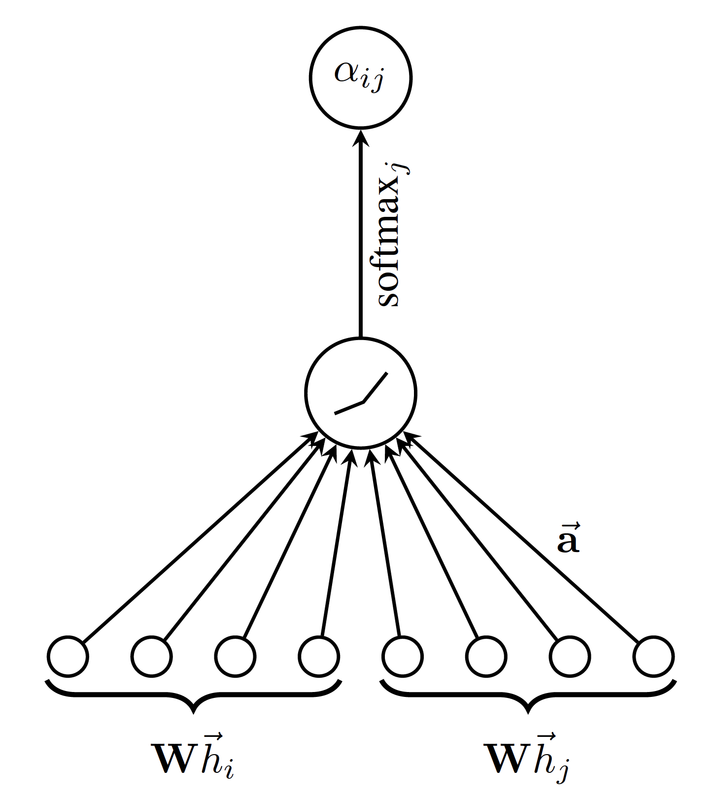
src: Veličković et al. 2018
Intuitively, $\overrightarrow{\mathbf{a}}^{T}\left[\mathbf{W} \vec{h}_{i} | \mathbf{W} \vec{h}_{j}\right]$ is a linear combination of transformed $h_i$ and $h_j$. It can be thought of as a distance between node $i$ and $j$ or some aggregate. (Answers Q-1)
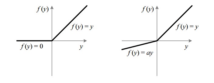
Since the slope of ReLU is zero for -ve values, the ability to train the model is compromised in that region. This is called dying ReLU problem. LeakyReLU activation function is used instead of ReLU with a=0.01 in the figure below to avoid that problem. LeakyReLU helps speed up learning and is more balanced. (Answers Q-2)
Following Vaswani et al. 2017, authors proposes to use $K$ independent attention mechanism to employ multi-head attention. So the mathematical form of each layer is:
$$ \vec{h}_{i}^{\prime}=\Biggm|_{k=1}^{K} \sigma\left(\sum_{j \in \mathcal{N}_{i}} \alpha_{i j}^{k} \mathbf{W}^{k} \vec{h}_{j}\right) $$
and the output $\mathbf{h}^{\prime}$ consists $K F^{\prime}$ features instead of $F^{\prime}$.
Only, in last layer the multi-head attentions are aggregated instead of concatenation. So, the mathematical form of last layer is:
$$ \vec{h}_{i}^{\prime}=\sigma\left(\frac{1}{K} \sum_{k=1}^{K} \sum_{j \in \mathcal{N}_{i}} \alpha_{i j}^{k} \mathbf{W}^{k} \vec{h}_{j}\right) $$
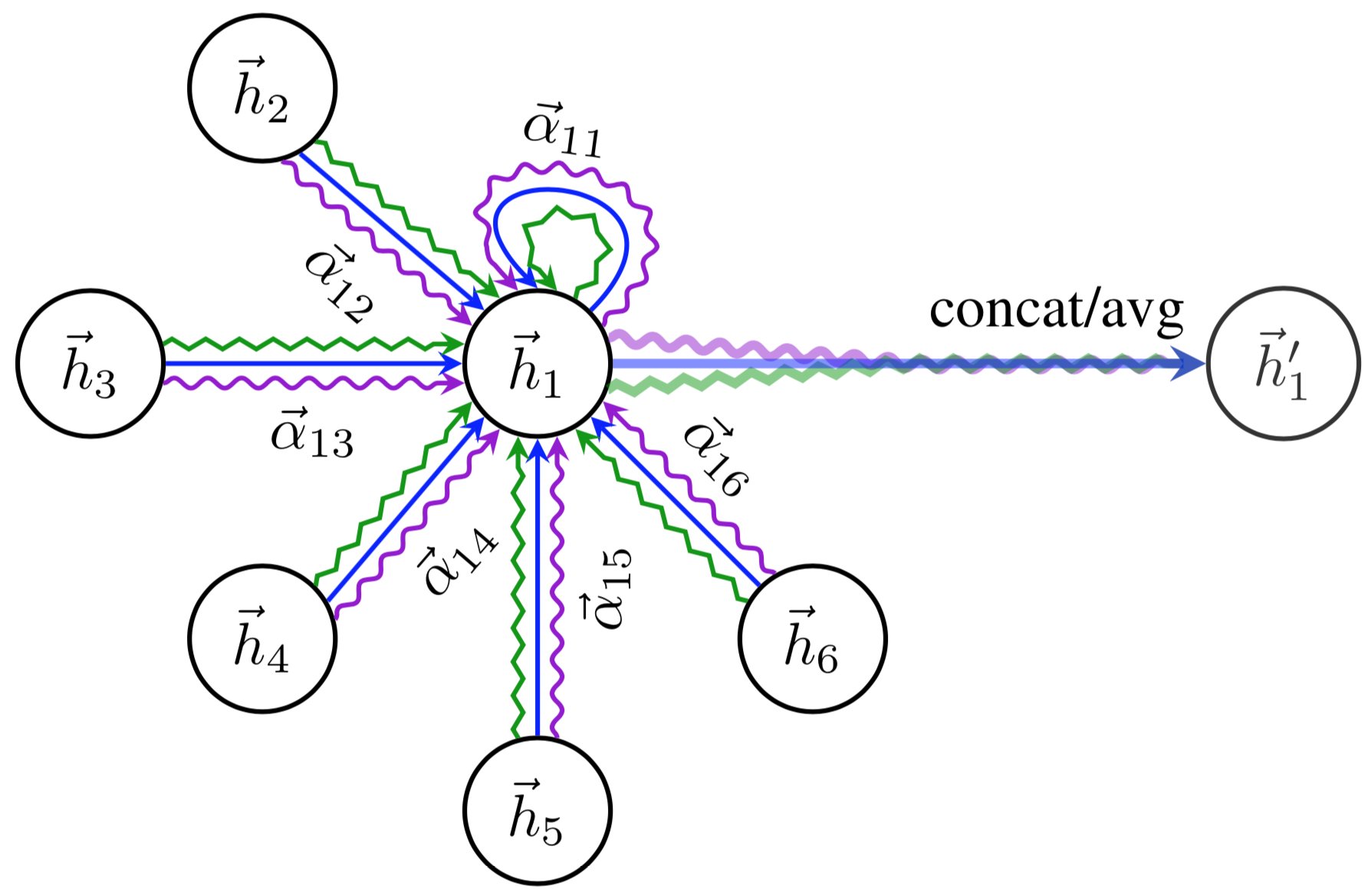
src: Veličković et al. 2018
Complexity
Time complexity of computing single attention head is sum of complexity of computing the $e_{i j}$ for each node and then computing the softmax. The feed forward neural network, computing $e_{i j} = \text{LeakyReLU}\left(\overrightarrow{\mathbf{a}}^{T}\left[\mathbf{W} \vec{h}_{i} | \mathbf{W} \vec{h}_{j}\right]\right)$ is effectively equivalent to complexity of matrix multiplication $\underbrace{\mathbf{W}}_{F^{\prime} \times F} \underbrace{\vec{h}_{i}}_{F \times 1} + \underbrace{\overrightarrow{\mathbf{a}}^{T}}_{1 \times 2F^{\prime}} \underbrace{\hat{h}}_{2F^{\prime} \times 1}$ for each node, $\mathcal{O}\left(|\mathcal{V}|(FF^{\prime} + 2F^{\prime})\right) = \mathcal{O}\left(|\mathcal{V}|FF^{\prime}\right)$, where $\mathcal{V}$ is number of nodes. Complexity of computing $\alpha_{i j} =\operatorname{softmax}_{j}\left(e_{i j}\right)$ for all the edges is $\mathcal{O}(|\mathcal{E}|F^{\prime})$, where $\mathcal{E}$ is number of edges. So, total complexity of a single attention head is $\mathcal{O}(|\mathcal{V}|FF^{\prime} + |\mathcal{E}|F^{\prime})$. (Answers Q-3)
Memory complexity of GAT for sparse matrix is linear in terms of nodes and edges. (Answers Q-4)
Experiments
Authors evaluate the GAT architecture for two type of learning tasks on graph structures:(Answers Q-5)
-
Transductive learning task is where the algorithm sees whole graph but labels of only few nodes are available. Algorithm is trained on these nodes and whole graph and the task is to produce labels for nodes which do not have labels while training. GCN works only for transductive setting.
-
Inductive learning task is when the algorithm sees only training nodes and edges between those nodes. Labels of all the training nodes are available and the task is to predict label for test nodes, which are unseen during training.
Transductive learning
For transductive learning task, 10 baseline architectures are compared (including GCN, MoNet, Chebyshev, MLP etc), for three datasets Cora, Citeseer and pubmed. Two layer GAT architecture was used as shown in figure below, with 8 attention heads in first layer and 1 attention head in second layer. Softmax was used in final layer and ELU activation is used in the first layer.
Mathematical form of the architecture:
$$ Z = \operatorname{softmax}\left( \tilde{A} \mathbf{\alpha}_{2}\mathbf{W}_2\left({\biggm|}_{k=1}^{8} \operatorname{ELU}\left(\tilde{A} \mathbf{\alpha}_{1}^{k}\mathbf{W}_1 H \right)\right) \right) $$
Inductive Learning
For inductive learning task, 6 baseline architectures are compared (including GraphSAGE, MLP etc), for PPI dataset. Three layer architecture was used as shown in the figure below.
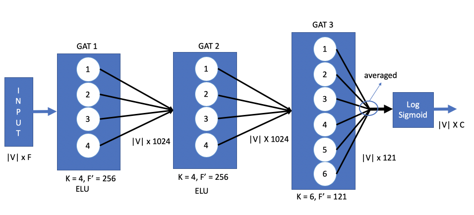
Mathematical form of the architecture:
$$ Z = \operatorname{LogisticSigmoid}\left( \frac{1}{6} \sum_{z=1}^{6} \tilde{A} \mathbf{\alpha}_{3}^{z}\mathbf{W}_3\left({\biggm|}_{y=1}^{4} \operatorname{ELU}\left(\tilde{A} \mathbf{\alpha}_{2}^{y}\mathbf{W}_2 \left({\biggm|}_{k=1}^{4} \operatorname{ELU}\left(\tilde{A} \mathbf{\alpha}_{1}^{k}\mathbf{W}_1 H \right) \right)\right)\right) \right) $$
Extensions
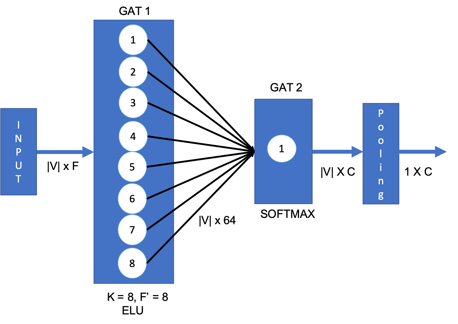
The GAT network can be extended to use for Graph classification by simply appending a pooling layer at the end. Figure below represents one such architecture.
GAT can also be used for embedding the nodes to two-dimensional space. One such architecture is presented below, where instead of Softmax, the last layer outputs 2-D vector for each node.
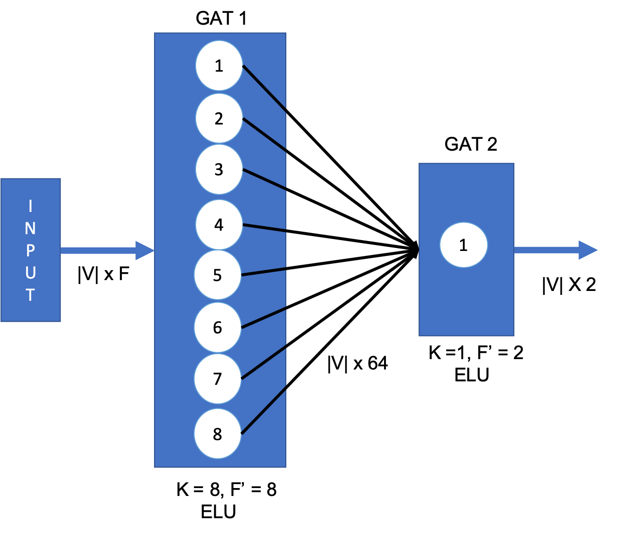
Mathematical form of this 2D embedding GAT network is
$$ Z = \operatorname{ELU}\left( \tilde{A} \mathbf{\alpha}_{2}\mathbf{W}_2\left({\biggm|}_{k=1}^{8} \operatorname{ELU}\left(\tilde{A} \mathbf{\alpha}_{1}^{k}\mathbf{W}_1 H \right)\right) \right) $$
Questions
- What attention mechanism is used in the experiments? Link to Answer
- Why LeakyReLU but not the standard ReLU ? Link to Answer
- Proof complexity of GAT layer is $O\left(|V| F F^{\prime}+|E| F^{\prime}\right)$. Link to Answer
- What is the memory complexity of GAT layer? Link to Answer
- Explain difference between transductive and inductive learning. Link to Answer
- Draw architecture of two layer GAT model for transductive learning. What is the Mathematical formulation? Link to Answer
- Draw architecture of three layer GAT model for inductive learning. What is the Mathematical formulation? Link to Answer
- Design a GAT model that embed the nodes of the cora network in a two-dimensional space. Draw the architecture and give the mathematic form. Link to Answer
- Design a GAT model for graph classification. Draw the architecture and give the mathematic form. Link to Answer
References
- Veličković, Petar, Guillem Cucurull, Arantxa Casanova, Adriana Romero, Pietro Lio, and Yoshua Bengio, Graph Attention Networks , ICLR 2018
- Graph Attention Networks overview by Peter Veličković
- ML Paper explained - AISC by Karim Khayrat: Graph Attention Networks Explained
- A Tutorial on Attention in Deep Learning, by Alex Smola and Aston Zhang, ICML 2019
- https://towardsdatascience.com/illustrated-self-attention-2d627e33b20a
- https://towardsdatascience.com/activation-functions-neural-networks-1cbd9f8d91d6
Previous post
Graph Convolutional Networks
Next post
Understanding Attention and Generalization in Graph Neural Networks