harsha kokel
Graph Convolutional Networks
My notes on Thomas N Kipf and Max Welling ICLR 2017. Written as part of the Complex Networks course by Prof. Feng Chen.
Introduction
Kipf et al. 2017 introduces Graph Convolutional Networks (GCN) which uses features of each node and leverages edges of the graph to derive class similarity between nodes in semi-supervised setting.
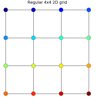
Traditionally semi-supervised learning in a graph-structured data heavily relied on the assumption that the edges in the graph represent class similarities (i.e. nodes with similar classes have edge between them). For example, in an image segmentation task, an image can be thought as a grid (Graph with node for every pixel and edges between neighboring pixels as shown in figure below). Such representation of an image represents the assumption that the neighboring pixels belong to the same class (hence an edge between them).
With this assumption, semi-supervised learning task is then posed as an optimization problem with following loss function:
\[ \mathcal{L}=\mathcal{L}_{0}+\lambda \mathcal{L}_{\mathrm{reg}}, \quad \text { with } \quad \mathcal{L}_{\mathrm{reg}}=\sum_{i, j} A_{i j}\left|f\left(X_{i}\right)-f\left(X_{j}\right)\right|^{2} \]
Here $\mathcal{L}_{0}$ is some form of cross-entropy loss for the supervised examples and the $\mathcal{L}_{\mathrm{reg}}$ is a regularizing function which tries to reduce difference in labels of connected nodes. $\mathcal{L}_{\mathrm{reg}}$ is laplacian quadratic form.
\[ \begin{aligned} f\left(X\right)^{\top} \Delta f\left(X\right) &= f\left(X\right)^{\top}(D-A) f\left(X\right) \\ &=f\left(X\right)^{\top} D f\left(X\right)-f\left(X\right)^{\top} A f\left(X\right) \\ &=\sum_{i=1}^{n} D_{ii} f\left(X_{i}\right)^{2}-\sum_{i=1}^{n} \sum_{j=1}^{n} A_{ij} f\left(X_{i}\right)f\left(X_{j}\right) \\ &=\sum_{i=1}^{n} \sum_{j=1}^{n} A_{ij} f\left(X_{i}\right)^{2}-\sum_{i=1}^{n} \sum_{j=1}^{n} A_{ij} f\left(X_{i}\right) f\left(X_{j}\right) \\ &=\sum_{i=1}^{n} \sum_{j=1}^{n} A_{ij}\left(f\left(X_{i}\right)^{2}-f\left(X_{i}\right) f\left(X_{j}\right)\right) \\ &=\sum_{{i, j} \in E}\left(f\left(X_{i}\right)-f\left(X_{j}\right)\right)^{2} \\ &= \sum_{i \leq j} A_{i j}\left|f\left(X_{i}\right)-f\left(X_{j}\right)\right|^{2} \end{aligned} \]
Graph Convolutional networks
GCN proposes a way to do graph convolutions by using the following layer wise propagation rule:
\[ \begin{aligned} H^{(l+1)} & =\sigma\left( \hat{A} H^{(l)} W^{(l)}\right), \\ \quad \text { with } \quad\hat{A} & = \tilde{D}^{-\frac{1}{2}}\tilde{A}\tilde{D}^{-\frac{1}{2}}, \\ \tilde{A} & = (A + I_{N}), \\ \end{aligned} \]
\[ \tilde{D_{ij}}=\left\{\begin{array}{ll}{\sum_{k=1}\tilde{A}_{ik},} & {\text { if } i = j} \\ { 0,} & {\text { otherwise }}\end{array}\right. \]
The paper proposes a two layer Graph Convolutional Network which amounts to following model:
\[ Z=f(X, A)=\operatorname{softmax}\left(\hat{A} \operatorname{ReLU}\left(\hat{A} X W^{(0)}\right) W^{(1)}\right) \]
- ReLU activation function is used in the first layer because the gradient of ReLU is $0/1$, so with multiple iterations, the gradient values do not vanish (tends to zero), which is the case with other non-linear functions. Softmax is used in the top layer, because the final output expected are class probabilities.
GCN uses gradient descent to learn weight matrices – $W^{(0)}$ and $W^{(1)}$ that minimizes the following cross-entropy error for all the supervised nodes ($\mathcal{Y}_{L}$):
\[ \mathcal{L}=-\sum_{l \in \mathcal{Y}{L}} \sum{f=1}^{F} Y_{l f} \ln Z_{l f} \]
Loss function is then a combination of cross-entropy loss for the supervised labels and some regularization.
\[ Loss=\mathcal{L} + \mathcal{L}_{reg}, \\ \begin{aligned} \text{with } \mathcal{L}_{reg} = & \frac{\lambda}{2} * \sum|W|^{2} \quad \text{ for L2-regularization} \\ & \frac{\lambda}{2} * \sum|W| \quad \text{ for L1-regularization} \end{aligned} \]
In the paper, authors observe that L2-regularization of weight matrix at the first layers alone is sufficient.
- Regularization is used to avoid overfitting by penalizing the weight matrices of hidden layers. L2-regularization in particular uses 2-norm of weight matrix for penalty. This pushes the weight matrix close to zero. (Answers Q-14)
Experiments
Connection between CNN and GCN
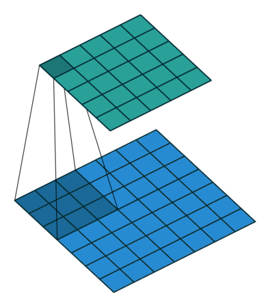
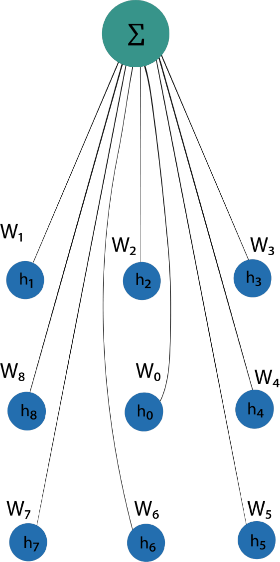
In CNN, input feature map (blue grid in below image) is convolved with discrete kernel ($W$) to produce output feature map (green grid). This can be seen as a message passing algorithm where the messages from the neighboring nodes ($h_i, i = 1 \text{ to } 8$ in the example below) and the node itself ($h_0$) are multiplied with weight $W_i$ and the output feature map is obtained by summing up these messages.
GCN similarly generates output feature map ($H^{(l+1)}$) by convolving the input feature map ($H^{(l)}$) with weight matrix ($W^{(l)}$).
\[ \begin{aligned} H^{(l+1)} & = \sigma\left( \hat{A} H^{(l)} W^{(l)}\right), \\ \text{ with } \quad \hat{A} & : n \times n \text{(\# nodes)}, \\ H^{(l)} & : n \times f^{i} \text{(\# input feature map)}, \\ W^{(l)} & : f^{i} \times f^{o} \text{(\# output feature map)}, \\ \end{aligned} \]
This can be seen as a message passing algorithm where messages or input features ($H_{ik}$) of each node in the graph are multiplied by weights ($W_{jk}$) and summation is stored in $B$ and finally, the output feature map ($M$) is generated by summing the weighted messages of all the neighboring nodes along with the message from the node itself (Note: $\tilde{A} = A + I_N$ takes care of message from node itself).
\[ \begin{aligned} M & = \hat{A} H^{(l)} W^{(l)} \\ & = \hat{A} B, \\ \text{ with } B_{ij} & = \sum_{k=1}^{f^{i}} H_{ik}W_{jk} \\ M_{ij} & = \sum_{k=1}^{n} \hat{A}{ik} B{kj} \end{aligned} \]
-
In CNN the number of neighbors for each node are fixed ($8$ in above example), so the number of messages received by all the nodes in the output later are same. In GCN, since the structure of graph is dictated by the adjacency matrix, the number of messages received at each node ($M_{ij}$) is not the same. Hence, the need for normalizing $\tilde{A}$ (i.e, $\hat{A} = \tilde{D}^{-\frac{1}{2}}\tilde{A}\tilde{D}^{-\frac{1}{2}}$) arises in GCN but not in CNN.
-
Although theoretically there are no limitations on number of convolution layers, GCN paper proposes two layered network. Since every layer convolves the neighboring node, $k$ layers effectively convolves $k^{th}$ order neighbors. GCN convolve only upto $2^{nd}$ order neighbors. Their empirical evaluations suggest 2nd order neighbor is enough for most of the domains. (Answers Q-13)
-
In traditional approach, since we use $\mathcal{L}_{reg}$, which is a function of adjacency matrix, the nodes with dense neighborhood will have high penalty and hence the model will overfit on the local neighborhoods of such nodes (consequently it will under-fit the nodes with sparse neighborhood). Normalization of adjacency matrix helps us alleviate this problem.
Extending GCN to graph classification and supervised learning task
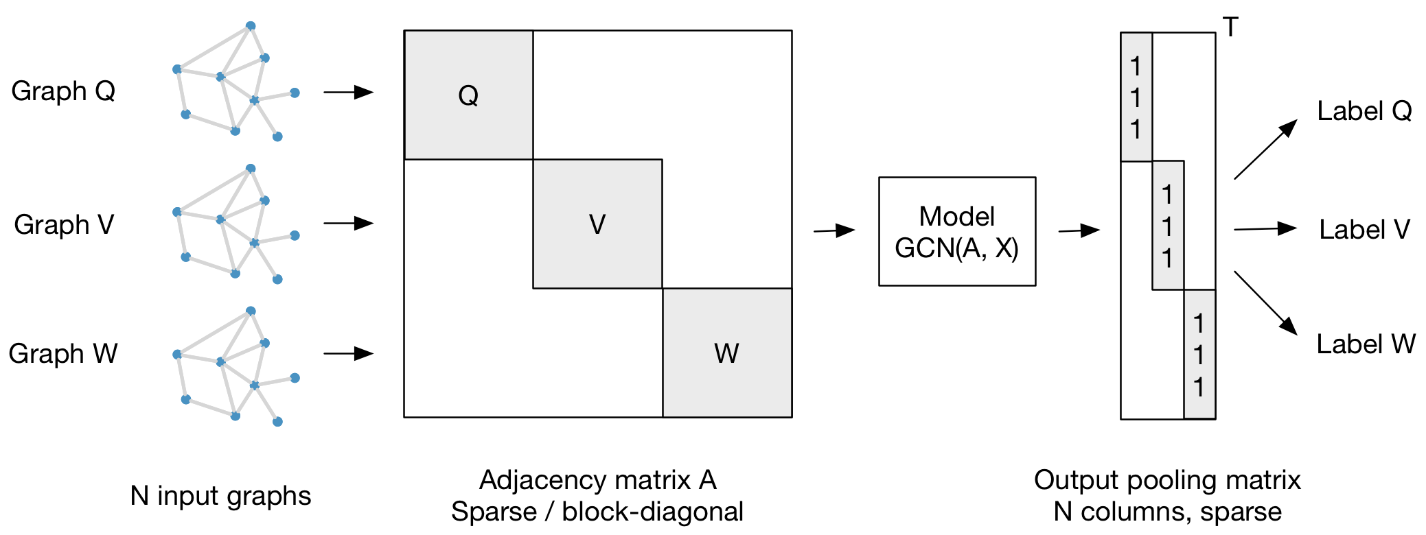
GCN formulation can be leveraged for graph classification problem, where the task is to predict a single variable for the whole graph. Adjacency matrix of each graph ($Q, V, W$ in the figure below) is concatenated into a sparse block-diagonal matrix ($A$) as shown in the figure below. This adjacency matrix and the feature matrix ($X: n \times c$, n = total number of nodes in all the graphs and c = # input features) can be used to train GCN and the output matrix Z can then be pooled to obtain class labels for each graph.
For supervised learning task, two graphs can be created from training set (labeled nodes) and the testing set (unlabeled nodes). Adjacency matrix of two graphs can again be concatenated as block-diagonal matrix and GCN can be trained on it. The output matrix Z will have the class probabilities for test set as well.
Spectral Graph Convolutions
Convolution theorem states that convolution of two matrices is equivalent to point-wise multiplication in the fourier domain i.e. $\mathcal{F}(x \ast y) = \mathcal{F}(x) \odot \mathcal{F}(y)$ when $\mathcal{F}(\ \ )$ denotes fourier transform operator. In signal processing, the spectral transformation usually refers to transformation from time to frequency dimension (fourier domain), but in graph theory spectral transformation usually refers transformation to eigen-vector dimension ($U^{\top}$). So, the convolution theorem in graphs represents following equation:
\[ \begin{aligned} \text{with } L & = U \Lambda U^{\top}, \\ \hat{\mathrm{x}} & = U^{\top}\mathrm{x}, \\ \hat{\mathrm{y}} & = U^{\top}\mathrm{y}, \\ U^{\top} (\mathrm{x} \ast \mathrm{y}) & = \hat{\mathrm{x}} \odot \hat{\mathrm{y}} \\ \mathrm{x} \ast \mathrm{y} = U ( \hat{\mathrm{x}} & \odot \hat{\mathrm{y}}) = U ({ \mathrm{diag}(\hat{\mathrm{y}})\hat{x}} ) \\ \mathrm{y} \ast \mathrm{x} = \mathrm{x} \ast \mathrm{y} = & U \ \mathrm{diag}(\hat{\mathrm{y}})\ U^{\top} \ \mathrm{x} \end{aligned} \]
- $\text {with } L = U \Lambda U^{\top}$ is eigen-decomposition of graph laplacian matrix. Complexity of finding eigen-decomposition if $\mathcal{O}(n^3)$ (Answers Q-2)
- Remember, matrix-vector multiplication ($A \mathrm{b}$) is effectively transformation of the vector ($b$) to another dimension dictated by the matrix ($A$).
- Since, L is a square matrix, $U^T = U^{-1}$.
For spectral graph convolution, we directly estimate the convolution filter in the eigen-vector dimension as some function of eigen-vectors ($\Lambda$). With filter $g_{\theta}(\Lambda) = \mathrm{diag}(\theta(\Lambda))$ spectral convolution on graph is defined as follows:
\[ g_{\theta}(\Lambda) \ \star \ \mathrm{x} = U g_{\theta}(\Lambda) U^{\top} \mathrm{x} \]
Note the difference between convolution symbol ($\ast$) and the spectral convolution symbol used in paper ($\star$) signifies that the $g_{\theta}$ is already in eigen-vector dimension.
$g_{\theta}$ can be approximated by truncated expansion in terms of Chebyshev polynomials $T_{k}(x)$ as:
\[ \begin{aligned} g_{\theta^{\prime}}(\Lambda) \approx \sum_{k=0}^{K} \theta_{k}^{\prime} T_{k}(\tilde{\Lambda}) \\ \text{ with } \quad \tilde{\Lambda}=\frac{2}{\lambda_{\max }} \Lambda-I_{N}, \\ T_{k}(x) = 2 x T_{k-1}(x)-T_{k-2}(x), \\ T_{0}(x)=1 \text { and } \quad T_{1}(x) =x \\ \end{aligned} \]
Chebyshev polynomial $T_{k}(\tilde{\Lambda})$ is a matrix with dimensions same as $\tilde{\Lambda}$ (i.e. $n \times n$, where n = # nodes ). Elements of matrix $T_{k}(\tilde{\Lambda})$ are obtained by applying Chebyshev polynomial definition element wise. (Answers Q-1)
So,
\[ \begin{aligned} T_0(\tilde{\Lambda}) & = \left[\begin{array}{cccc}{T_{0}\left(\frac{2}{\lambda_{\max }}\left(\lambda_{1}-1\right)\right)} & {} & {} & {} \ {} & {T_{0}\left(\frac{2}{\lambda_{\max }}\left(\lambda_{2}-1\right)\right)} & {} & {} \ {} & {} & {\ddots} & {} \ {} & {} & {} & {T_{0}\left(\frac{2}{T_{\max }}\left(\lambda_{N}\right)\right)}\end{array}\right] \\ & = \left[ \begin{array}{cccc}{1} & {} & {} & {} \\ {} & {1} & {} & {} \\ {} & {} & {\ddots} & {} \\ {} & {} & {} & {1}\end{array} \right] \\ & = I_N \\ \\ & \therefore\boxed{ \quad T_{0}(\tilde{\Lambda})= I_N \text{ and } T_{1}(\tilde{\Lambda}) =\tilde{\Lambda} } \end{aligned} \]
Observe that $\left(U \Lambda U^{\top}\right)^{k}=U \Lambda^{k} U^{\top}$ and $U T_{k}(\tilde{\Lambda}) U^{\top} = T_{k}(\tilde{L})$.
Proofs (Answers Q-4): \[ \begin{aligned} (U \Lambda U^{\top})^{2} & = ( U \Lambda U^{\top} )( U \Lambda U^{\top} ) \\ & = U \Lambda ( U^{\top} U ) \Lambda U^{\top} \\ & = U \Lambda I \Lambda U^{\top} \\ & = U \Lambda ^{2} U^{\top} \\ \end{aligned} \] \[ \text{ Similarly, } \boxed{ \left(U \Lambda U^{\top}\right)^{k}=U \Lambda^{k} U^{\top} } \]
and
\[ \begin{aligned} {U T_{0}(\tilde{\Lambda}) U^{\top}=U I_{N} U^{\top}=I_{N}=T_{0}(\tilde{L})}, \\ {U T_{1}(\tilde{\Lambda}) U^{\top}=U \tilde{\Lambda} U=\tilde{L}=T_{1}(\tilde{L})}, \\ \end{aligned} \] \[ \begin{aligned} U T_{2}(\tilde{\Lambda}) U^{\top} & = U \Big(2 \tilde{\Lambda} T_{1}(\tilde{\Lambda})- T_{0}(\tilde{\Lambda}) \Big) U^{\top} \\ & = 2 U \tilde{\Lambda} T_{1}(\tilde{\Lambda}) U^{\top}- U T_{0}(\tilde{\Lambda}) U^{\top} \\ & = 2 U \tilde{\Lambda} U^{\top} U T_{1}(\tilde{\Lambda}) U^{\top}- U T_{0}(\tilde{\Lambda}) U^{\top} \\ & = 2 \tilde{L} T_{1}(\tilde{L}) - T_{0}(\tilde{L})\\ & = T_2(\tilde{L}) \\ \end{aligned} \] \[ \text{ Similarly, } \boxed { U T_{k}(\tilde{\Lambda}) U^{\top} = T_{k}(\tilde{L}) } \\ \]
Using the above two results, we can approximate the convolution without needing eigen-decomposition, directly using graph laplacian,
\[ \begin{aligned} g_{\theta^{\prime}}(\Lambda) \star x & \approx U \sum_{k=0}^{K} \theta_{k}^{\prime} T_{k}(\tilde{\Lambda}) U^{\top} \mathrm{x} \\ & = \sum_{k=0}^{K} \theta_{k}^{\prime} U T_{k}(\tilde{\Lambda}) U^{\top} \mathrm{x} \\ & = \sum_{k=0}^{K} \theta_{k}^{\prime} T_{k}(\tilde{L}) \mathrm{x} \end{aligned} \]
So, we effectively reduced the complexity of convolution from $\mathcal{O}(n^3)$ to $\mathcal{O}(|\mathcal{E}|)$, i.e. from cube of # nodes ($n$) to linear in # edges ($\mathcal{E}$). Since $T_i(\tilde{L})$ has $2\mathcal{E}$ non-zero elements, multiplication $\underbrace{\theta_k^{\prime}}_{scalar} \underbrace{T_i(\tilde{L})}_{n \times n} \underbrace{\mathrm{x}}_{n \times 1}$ is a sparse matrix multiplication which can be done in $\mathcal{O}(|\mathcal{E}|)$. (Answers Q-5):
Connection between GCN and spectral convolutions
GCN can be seen as approximation of spectral convolution with $K = 1$, $\lambda_{max}=2$ and $\theta = \theta_0^{\prime} = - \theta_1^{\prime}$ (Answers Q-8)
\[ \begin{aligned} g_{\theta^{\prime}}(\Lambda) \star x & \approx \sum_{k=0}^{1} \theta_{k}^{\prime} T_{k}(\tilde{L}) x \\ & = \theta_{0}^{\prime} T_{0}(\tilde{L}) x+\theta_{1}^{\prime} T_{1}(\tilde{L}) x\\ & = \theta_{0}^{\prime} I_{N} x+\theta_{1}^{\prime}\left(\frac{2}{\lambda_{\max }} L-I_{N}\right) \\ & =\theta_{0}^{\prime} x+\theta_{1}^{\prime}\left(L-I_{N}\right) \quad \boxed{\because \lambda_{max}=2} \\ & =\theta_{0}^{\prime} x-\theta_{1}^{\prime} D^{-\frac{1}{2}} A D^{-\frac{1}{2}} \quad \boxed{\because L=I_{N}-D^{-\frac{1}{2}} A D^{-\frac{1}{2}}} \\ & = \theta \left(I_{N}+D^{-\frac{1}{2}} A D^{-\frac{1}{2}}\right) x \quad \boxed{\because \theta = \theta_0^{\prime} = - \theta_1^{\prime}} \\ & = \theta \left(\tilde{D}^{-\frac{1}{2}} \tilde{A} \tilde{D}^{-\frac{1}{2}}\right) x \quad \boxed{ \because \underbrace{I_{N}+D^{-\frac{1}{2}} A D^{-\frac{1}{2}} \rightarrow \tilde{D}^{-\frac{1}{2}} \tilde{A} \tilde{D}^{-\frac{1}{2}}}{\text{renormalization trick }}, \text { with } \tilde{A}=A+I{N} } \\ & = \theta \hat{A} x \end{aligned} \]
If we use convolution formula $g_{\theta} \star x \approx \theta\left(I_{N}+D^{-\frac{1}{2}} A D^{-\frac{1}{2}}\right) x$ repeatedly over multiple layers, values keep increasing in every layer since we have $I_N$. Renormalization trick is used to avoid this. (Answers Q-9 and 10)
Since GCN uses $K =1$ and approximates $\theta = \theta_0^{\prime} = - \theta_1^{\prime}$, which reduces the number of parameters we intuitively determine that GCN will not overfit the graphs. (Answers Q-6)
When we use $\theta = \theta_0^{\prime} = - \theta_1^{\prime}$ we are assigning same weights to all the 1st and 2nd order neighbors. If we used different $\theta$, we will assign different weights to different hop neighbors.
Renormalization Trick: With $I_{N}+D^{-\frac{1}{2}} A D^{-\frac{1}{2}}$, the eigen values are in range [0,2]. When the largest eigenvalue is less than $1$ the vanishing problem may occur even in case of two layers. With the renormalization trick, we can ensure that the eigen values are between [0,1] and the maximum eigenvalue is $1$. So, we avoid vanishing problem.
So, \[ \begin{aligned} g_{\theta^{\prime}}(\Lambda) \star x & = diag(\theta) T_{k}(\tilde{L}) X \\ & = T_{k}(\tilde{L}) \ X \ diag(\theta) \end{aligned} \]
Since this will still give us $n \times f^{i}$ matrix, we add a weight matrix ($W^{\prime}_{f^{i} \times f^{o}}$) to linearly transform the result to $n \times f^{o}$
So, \[ \begin{aligned} g_{\theta^{\prime}}(\Lambda) \star x & = T_{k}(\tilde{L}) \ X \ diag(\theta) \ W^{\prime} \\ & = \hat{A} X W \end{aligned} \]
With $X \in \mathbb{R}^{n \times f^{i}}$, we have $\underbrace{Z}_{n \times f^{o}} = \underbrace{\hat{A}}_{n \times n} \underbrace{X}_{n \times f^{i}} \underbrace{W}_{f^{i} \times f^{o}}$ which is graph convolution. Complexity of matrix multiplication is $\mathcal{O}(n f^{i}f^{o})$ since $\hat{A}$ is a sparse matrix with $\mathcal{E}$ non-zero elements – Not sure how paper gets $\mathcal{O}(|\mathcal{E}| f^{i}f^{o})$ (Answers Q-12)
Limitations
-
GCN provides equal importance to self node as well as the neighboring introduces. It also does not allow to different weights for different neighbors, which is allowed in CCN.
-
GCN being a graph convolution in the spectral domain, the Graph structure if fixed. Spatial domain convolutions on other hand allow for graph modifications.
-
Although GCN considers node features, it still heavily rely on the node locality.
Questions
-
What is the dimensionality of $T_{k}(\tilde{\Lambda})$, how to calculate $i^{th}$ row and $j^{th}$ column of matrix $T_{k}(\tilde{\Lambda})$? Link to Answer
-
What is the time complexity to compute the eigen-decomposition Link to Answer
-
What is the relation between $g \star x$ and GCN? Link to Answer
-
Prove $\left(U \Lambda U^{\top}\right)^{k}=U \Lambda^{k} U^{\top}$. Link to Answer
-
Prove complexity of $\sum_{k=0}^{K} \theta_{k}^{\prime} T_{k}(\tilde{L}) x$ is $\mathcal{O}(|\mathcal{E}|)$. Link to Answer
-
Describe the intuition, why GCN can alleviate the problem of overfitting on local neighborhood structures for graphs with very wide node degree distributions? Link to Answer
-
Why is $\lambda_{max} = 2$ a valid approximation?
Probably because eigen values of A $\in$ [0,1] and $\lambda_{max}$ is the eigen value of $A + I_N$, so the eigen values are in range [0,2]. We need this rescaloing because the Chebyshev polynomial needs input in range [-1,1]
-
Prove $g_{\theta^{\prime}} \star x \approx \theta_{0}^{\prime} x+\theta_{1}^{\prime}\left(L-I_{N}\right) x$. Link to Answer
-
Why does repeated application of $g_{\theta} \star x \approx \theta\left(I_{N}+D^{-\frac{1}{2}} A D^{-\frac{1}{2}}\right) {x}$ result in numerical instability? Link to Answer
-
Why does renormalization trick help? Link to Answer
-
Show in detail how to apply GCN for graph classification and supervised learning problem? Link to Answer
-
Derive time and memory complexity of $Z=\tilde{D}^{-\frac{1}{2}} \tilde{A} \tilde{D}^{-\frac{1}{2}} X \Theta$ Link to Answer
-
Why use 2 layers in GCN? Link to Answer
-
Explain L-2 regularization. Link to Answer
References
- Thomas N Kipf and Max Welling, Semi-supervised classification with Graph Convolutional Networks, ICLR 2017
- Notes by Prof. Feng Chen
- https://tkipf.github.io/graph-convolutional-networks/
- Ferenc Huszár’s GCN post
- https://dtsbourg.me/thoughts/posts/semi-supervised-classification-gcn
- https://medium.com/@BorisAKnyazev