
harsha kokel
Fitted Q and Batch Reinforcement Learning
Some pointers on Batch Reinforcement Learning and Fitted Q. These were gathered while working on an RL for healthcare project, as part of Advanced RL course by Prof. Sriraam Natarajan.
Terminologies
Offline Planning Problem (MDP)
We are given the full MDP model and the problem is solved using all the components of the MDP
Online Planning Problem (RL)
We have limited knowledge of the MDP. We can discover it by interacting with the system
Model-based RL
Approaches to solving Online planning problem (RL) by first estimating (when missing) or accessing the full MDP Model i.e. transition and reward function and then finding policy $\pi$ is called Model-based RL
Model-free RL
On the contrary, approaches to solving the Online RL Problem directly, i.e. solving for $\pi$ directly with either value function $V$ or state-action function $Q$ is called Model-free RL.
Batch RL
The simulation environment is not present and complete set of transition samples $\langle s, a, r, s^{\prime} \rangle$ is given and the challenge is to learn without exploring.
Background on Q Learning
Bellman optimality equation for the action-value function ($Q$) is given as:
$$Q^{\pi}(s, a)=\sum_{s^{\prime}} T\left(s, a, s^{\prime}\right)\left[R\left(s, a, s^{\prime}\right)+\gamma \sum_{a^{\prime}} \pi\left(s^{\prime}, a^{\prime}\right) Q^{\pi}\left(s^{\prime}, a^{\prime}\right)\right] $$
where $T\left(s, a, s^{\prime}\right)$ is a transition probability of landing in state $s^{\prime}$ on taking action $a$ in state $s$ and $R\left(s, a, s^{\prime}\right)$ is a Reward at state $s^{\prime}$ reached on taking action $a$ in state $s$.
In the dynamic programming setting, the $Q$ function for optimal policy is represented as:
$$Q_{k+1}(s, a) \leftarrow \sum_{s^{\prime}} T\left(s, a, s^{\prime}\right)\left[R\left(s, a, s^{\prime}\right)+\gamma \max {a^{\prime}} Q{k}\left(s^{\prime}, a^{\prime}\right)\right] $$
Q-Learning is a model-free approach to learn the $Q$ function by exploring the environment, i.e. performing actions based on some policy. A table of Q function for each state action pair $Q(s,a)$ is maintained and the table in updated after every action using the running average formula:
$$Q(s, a) \leftarrow(1-\alpha) Q(s, a)+(\alpha)[ R\left(s, a, s^{\prime}\right)+\gamma \max_{a^{\prime}} Q\left(s^{\prime}, a^{\prime}\right)] $$
With multiple episodes the Q values will eventually converge and the optimal policy might be retrieved from that.
Drawbacks of Q Learning.
There are several draw backs of the Q-Learning. These drawbacks might be minor in typical reinforcement learning setting where we have simulators. But these drawbacks are serious limitations in the Batch RL setting. In Batch RL, the simulation environment is not present and complete set of transition samples ($\langle s, a, r, s^{\prime} \rangle$) is given and the challenge is to learn without exploring.
Exploration overhead
As we see it in the figure below, at some point in the top left cell $(1,3)$, agent explored the action of going north and because it landed in the same cell, it updated $Q(s,north)=0.11$ as per the $\max_{a} Q(s,a)$ of that cell during that episode. After that episode, even though the $\max_{a} Q(s,a)$ of that cell changes, the $Q(s,north)$ does not get updated till the agent explores going north.
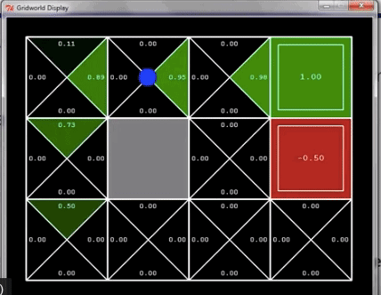
source: UC Berkeley CS188: Lecture of Pieter Abbeel
Stability issue
Q-Learning has ‘asynchronous update’ i.e. after each observation the value is updated locally only for the state at hand and all other states are left untouched. In the above figure, we know the value at the Red tile, but the Q value for the tile below it is not updated until we explore the action of going to red tile from that tile.
Similar idea of asynchronous update is also applicable in function approximations where $Q$ function is estimated by a function and at every time step the function is updated using:
$$f(s, a) \leftarrow(1-\alpha) f(s, a)+\alpha \left( r +\gamma \max_{a^{\prime} \in A} f\left(s^{\prime}, a^{\prime}\right) \right) $$
Inefficient approximation
The ‘asynchronous update’ in function approximation is particularly harmful with global approximation functions. An attempt to improve $Q$ value of a single state after every time step might impair all other approximations. Specially when approximation function used is like Neural Network, where a single example can impact changes in all the weights. Gordon 1995 proves that using an impaired approximation in next iteration, the $f$ function may divergence from the optimal $Q$ function.
This is where fitted methods come in.
Fitted Approaches
Gordon 1995 provided a stable function approximation approach by separating dynamic programming step from function approximation step. Effectively, the above function update equation is now split to two steps.
$$f^{\prime}(s, a) \leftarrow r +\gamma \max_{a^{\prime} \in A} f\left(s^{\prime}, a^{\prime}\right) , , , , \forall s,a \\ f(s, a) \leftarrow(1-\alpha) f(s, a)+\alpha f^{\prime}(s, a) $$
Observation: Splitting the function update from one to two steps is equivalent to changing the gram-schmidt orthonormalization to modified-gram schmidt orthonormalization.
Ernst 2005 proposed fitted Q iteration by borrowing the splitted approach from Gordon. The approach proposes iterative approximation of Q value by reformulating the Q Learning as a supervised regression problem. Algorithm proposed for fitted Q iteration is mentioned below.
Given: tuples {<s,a,r,s'>}, stopping condition

1. Q(s, a) = 0
2. while (!stopping condition):
3.    Build a training set:
         {feature; regression value} = {<s,a> ; r + max_a Q(s,a)}
4.    Learn a function approximating the regression values Q (s,a)
This is in principle similar to equations mentioned above, with $f^{\prime}$ as regression value and $\alpha=1$.
Further extensions to the fitted Q approaches have learnt $f$ function as some linear combination of the previous function and regression values.
References
- Lange, S., Gabel, T., & Riedmiller, M. Batch Reinforcement Learning. 2012
- Gordon, G. J. Stable Function Approximation in Dynamic Programming, ICML 1995.
- Ernst, D., Geurts, P., & Wehenkel, L. Tree-Based Batch Mode Reinforcement Learning, In JMLR 2005.
- http://www.cs.toronto.edu/~zemel/documents/411/rltutorial.pdf