harsha kokel
Few-Shot Learning with GNN
My notes on Victor Garcia, Joan Bruna, ICLR 2018. Written as part of the Complex Networks course by Prof. Feng Chen.
This paper focuses on $q$-shot $K$-way classification problem – where we have $K$ class labels and for each class label we have $q$ example images, so totally we have $s=qK$ training images. Authors propose to leverage the progress in Graph Convolutional Networks by formulating this problem as a node classification problem in graph $(G=(V,E))$, where nodes are images and an edge between two nodes indicate those two images are similar and may have same labels.
Given dataset $\{\left(\mathcal{T}_{i}, y_{i}\right)\}_{i\leq L}$ containing Task $\mathcal{T}_i$ and true label $y_{i} \in\{1, K\}$ for a single test image $\bar{x}$.
$$ \mathcal{T}=\left\{ \underbrace{ \left\{\left(x_{1}, l_{1}\right), \ldots\left(x_{s}, l_{s}\right)\right\}}_{\text{supervised samples}}, \underbrace{\left\{\bar{x}\right\}}_{\text{test samples}} ; \right\} $$
Embeddings$-\phi(.)$ are obtained from a convolutional neural network (CNN) for all the images ($\{x_i\}_1^s \cup \bar{x}$), as highlighted in the image below.
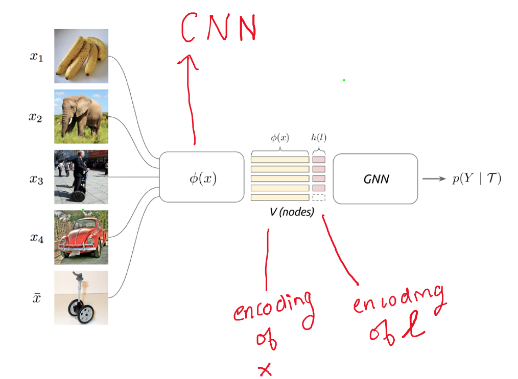
These embeddings are then concatenated with one-hot encoding of the labels $(h(l))$. Together they form nodes $(V)$ of the graph.
$\mathbf{x}_{i}^{(0)}=\left(\phi\left(x_{i}\right), h\left(l_{i}\right)\right)$
For $k$ labels, $h(l)$ is a binary vector of size k. One-hot encoding is obtained for training image $x_i$ with the label $l_i=3$, by setting all the values in $h(l_i)$ to $0$ except for $3^{rd}$ element which is $1$ i.e. $[0,0,1,0,0…]$. For test image, since the label is not known in $\mathcal{T}$, uniform distribution is used instead of one hot encoding i.e. $h(l) = k^{-1}\mathbf{1}_k$, for $\bar{x}$.
superscript $^{(p)}$ indicate the $(p+1)^{th}$ layer input. So, $x^{(0)}$ indicates the node embeddings for first layer in GNN.
Edges $(E)$ of the graph are learnt as adjacency matrix $\tilde{A}$ using a MLP.
$$ \tilde{A}_{i,j} = \varphi_{\tilde{\theta}}\left(\mathbf{x}_{i}, \mathbf{x}_{j}\right)= \operatorname{MLP}_{\tilde{\theta}}\bigg( \operatorname{abs}\Big( \phi(x_i) - \phi(x_j) \Big) \bigg) $$
Then Graph Convolution ($Gc(.)$) is performed on the nodes $V$ and adjacency matrix $A$. .
$$ \mathbf{x}_{l}^{(k+1)}=\operatorname{Gc}\left(\mathbf{x}^{(k)}\right)=\rho\left(\sum_{B \in \mathcal{A}} B \mathbf{x}^{(k)} \theta_{B, l}^{(k)}\right) \\ \mathcal{A} = \{\tilde{A}^{(k)}, \mathbf{1}\} $$
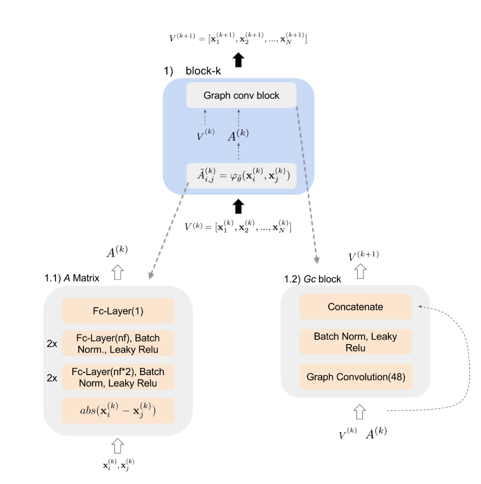
Proposed block of GNN containing the Adjacency matrix and Graph Convolution.
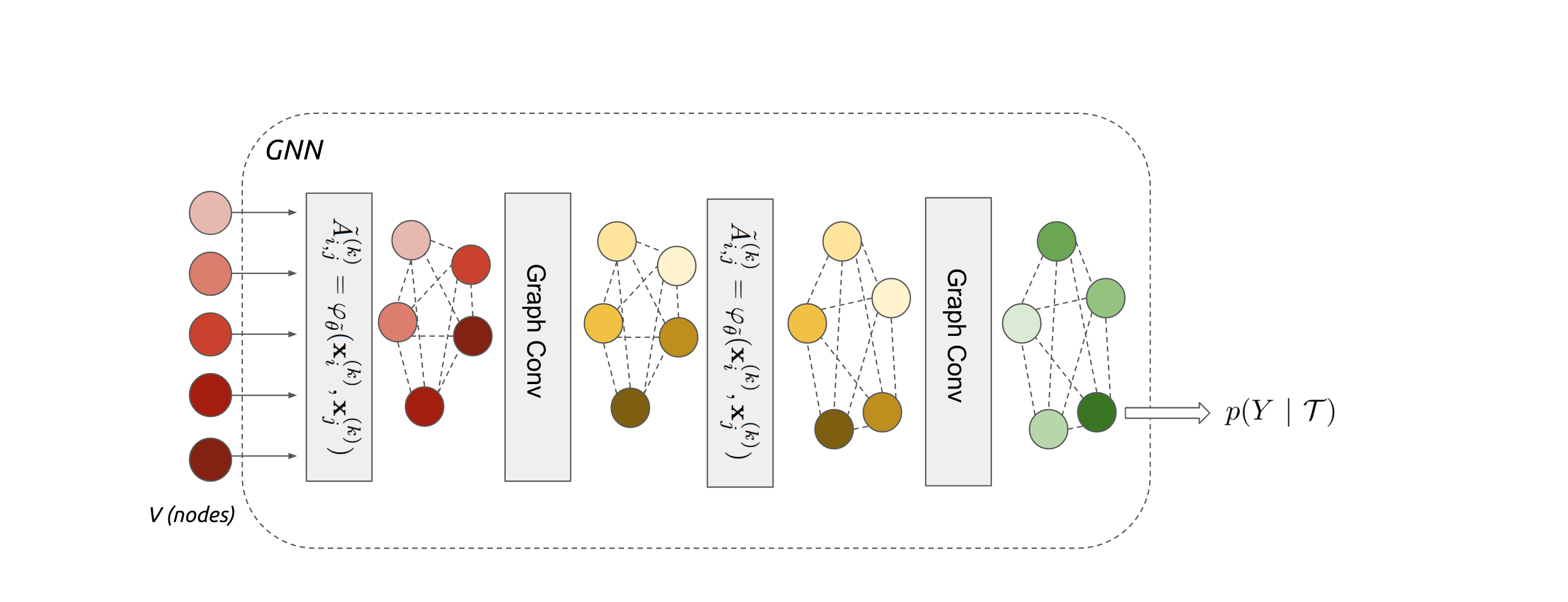
The block containing learning of adjacency matrix and graph convolution is repeated multiple times in the experiments and output of the last layer is passed through a sigmoid activation function to obtain class probabilities .
The complete network, including the adjacency matrix is trained end-to-end with following objective .
$$ \min _{\Theta} \frac{1}{L} \sum_{i \leq L} \underbrace{\ell\left(\Phi\left(\mathcal{T}_{i} ; \Theta\right), Y_{i}\right)}_{\text{loss w.r.t. test samples}}+\underbrace{\mathcal{R}(\Theta)}_{\text{regularizer}} \\ \ell(\Phi(\mathcal{T} ; \Theta), Y)= \underbrace{-\sum_{k} y_{k} \log P\left(Y=y_{k} | \mathcal{T}\right)}_{\text{cross entropy loss}} $$
Note that the labels/predictions of the training data are not used to compute the loss. Hence the GNN will not overfit to the $h(l)$ part of the embedding.
The over all idea of finding image embeddings and then using distance between the image embeddings to find the class label is explored in various other papers. Authors show equivalence of their approach to three other papers.
1. Convolutional Siamese Neural Network
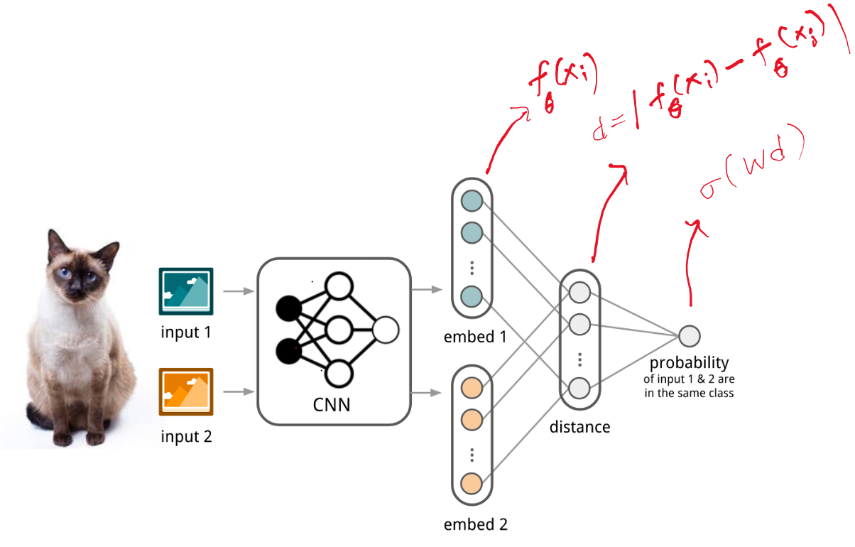
Koch et al. 2015 proposed to use Convolutional Siamese Neural Network (CSNN) to learn similarity between two images, i.e probability that both images were drawn from same label set.
They used two parallel twin CNN to obtain embeddings to two input images $f_{\theta}(x)$, computed absolute distance between these embeddings (d), and then computed probability by passing the distance from linear feedforward layer and sigmoid function.
CSNN are trained to reduce the following loss function for all pairs of images.
$$ \mathcal{L}(B)=\sum_{\left(\mathbf{x}_{i}, \mathbf{x}_{j}, y_{i}, y_{j}\right) \in B} \mathbf{1}_{y_{i}=y_{j}} \log p\left(\mathbf{x}_{i}, \mathbf{x}_{j}\right)+\left(1-\mathbf{1}_{y_{i}=y_{j}}\right) \log \left(1-p\left(\mathbf{x}_{i}, \mathbf{x}_{j}\right)\right) $$
While testing, the test image ($\mathbf{x}$) is compared with all the training images ($S$) and 1 Nearest-Neighbour approach is used to assign the class label.
$$ \hat{c}_{S}(\mathbf{x})=c\left(\arg \max _{\mathbf{x}_{i} \in S} P\left(\mathbf{x}, \mathbf{x}_{i}\right)\right) $$
Equivalence to GNN
GNN approach is similar to CSNN if we make following changes:
- Restrict node embeddings:
$$\operatorname{GNN}: \mathbf{x}_{i}^{(0)}=\left(\phi\left(x_{i}\right), h\left(l_{i}\right)\right)$$ $$\operatorname{CSNN}: \mathbf{x}_{i}^{(0)}=\phi\left(x_{i}\right) = f_{\theta}(x_i)$$
- Fix Adjacency matrix:
$$\operatorname{GNN}: \tilde{A}_{i,j} = \operatorname{MLP}_{\tilde{\theta}}\bigg( \operatorname{abs}\Big( \phi(x_i) - \phi(x_j) \Big) \bigg)$$ $$\operatorname{CSNN}: \tilde{A}_{i,j} = \operatorname{softmax}\bigg( - || \phi(x_i) - \phi(x_j) || \bigg)$$
- Reduce the convolution block:
$$\operatorname{GNN}: y = \sigma \Big( \sum_{B \in A} B \mathbf{x}^{(k)} \theta_{B,l}^{(k)} \Big)$$ $$\operatorname{CSNN}: Y_{\ast} = \sum_{j} \tilde{A}_{\ast, j}^{(0)}\left\langle\mathbf{x}_{j}^{(0)}, u\right\rangle$$
where, $\langle .,. \rangle$ indicates elementwise multiplication and $u$ is a binary vector for selection of labels. So, it is 1 only for elements which correspond to labels in $\mathbf{x}$ and 0 otherwise. $\{\ast\}$ indicates the test example. .
2. Matching Network
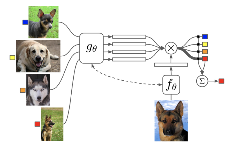
Vinyals et al., 2016 extended the SCNN approach of $2$-way comparison to $k$-way comparison by using an attention function $a(.,.)$ to compute cosine similarity of test image embedding $f_{\theta}(\mathbf{x})$ with input image embeddings $g_{\theta}(\mathbf{x_i})$ and use it as a weighted sum to compute the class probability of the test image.
$$ c_{S}(\mathbf{x})= P(y | \mathbf{x}, S)=\sum_{i=1}^{k} a\left(\mathbf{x}, \mathbf{x}_{i}\right) y_{i}, \text { where } S=\left\{\left(\mathbf{x}_{i}, y_{i}\right)\right\}_{i=1}^{k} a\left(\mathbf{x}, \mathbf{x}_{i}\right)= \frac{\exp \left(\operatorname{cosine}\left(f(\mathbf{x}), g\left(\mathbf{x}_{i}\right)\right)\right.}{\sum_{j=1}^{k} \exp \left(\operatorname{cosine}\left(f(\mathbf{x}), g\left(\mathbf{x}_{j}\right)\right)\right.} $$
Note here $k$ is the number of examples not the number of class labels.
Parameters $\theta$ are trained to maximize the loglikelihood of the test images.
$$ \theta=\arg \max _{\theta} E_{L \sim T}\left[E_{S \sim L, B \sim L}\left[\sum_{(x, y) \in B} \log P_{\theta}(y | x, S)\right]\right] $$
Equivalence to GNN
GNN approach can be considered equivalent to Matching Network if $f = g$ and $\mathbf{x}_{i}^{(0)}=\phi\left(x_{i}\right) = f_{\theta}(x_i)$ and $A_{i,j} = a(\mathbf{x_i, x_j})$.
2. Prototypical Network
Snell et al. 2017 reduced the number of comparisons in Matching Network by computing a class representative for each class and instead of comparing with all available images, the test image is only compared with the class representatives.
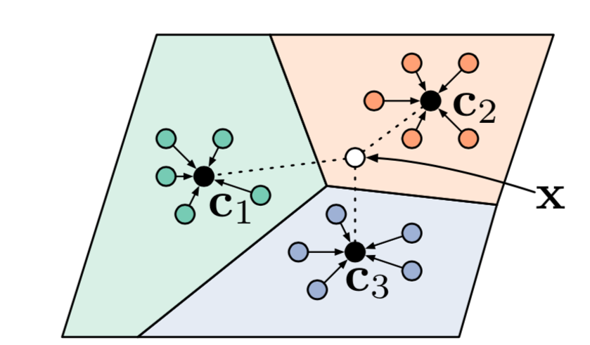
This paper first computes embeddings of all images $f_{\theta}(x_i)$ and then computes a class representative/prototype $\mathbf{v}_c$ for each class as mean of those embeddings.
$$ \mathbf{v}_{c}=\frac{1}{\left|S_{c}\right|} \sum_{\left(\mathbf{x}_{i}, y_{i}\right) \in S_{c}} f_{\theta}\left(\mathbf{x}_{i}\right) $$
The class probability distribution of test example is then computed by taking softmax of the distance between the embedding of test image and the class prototype. The distance measure used here is squared euclidean distance.
$$ P(y=c | \mathbf{x})=\operatorname{softmax}\left(-d_{\varphi}\left(f_{\theta}(\mathbf{x}), \mathbf{v}_{c}\right)\right)=\frac{\exp \left(-d_{\varphi}\left(f_{\theta}(\mathbf{x}), \mathbf{v}_{c}\right)\right)}{\sum_{c^{\prime} \in \mathcal{C}} \exp \left(-d_{\varphi}\left(f_{\theta}(\mathbf{x}), \mathbf{v}_{c^{\prime}}\right)\right)} $$
The network is trained to reduce the negative loglikelihood.
$$\mathcal{L}(\theta)=-\log P_{\theta}(y=c | \mathbf{x})$$
Equivalence to GNN
GNN approach can be reduced to Prototypical Network if we make following changes.
-
Restrict the node embeddings to $\mathbf{x}_{i}^{(0)}=\phi\left(x_{i}\right) = f_{\theta}(x_i)$
-
Fix the Adjacency Metric:
$$ \tilde{A}_{i, j}^{(0)}=\left\{\begin{array}{cc} q^{-1} & \text {if } l_{i}=l_{j} \\ 0 & \text{ otherwise } \end{array}\right. $$
q is the number of examples in each class.
- Replace the convolution block by:
$$\hat{Y}_{\ast}=\sum_{j} \tilde{A}_{\ast, j}^{(0)}\left\langle\mathbf{x}_{j}^{(0)}, u\right\rangle$$
Extentions
Paper also proposed a way to extend the few-shot learning setting to semi-supervised learning and active learning setting. Although straight forward I do not see the intuition clear enough or experiments strong enough to suggest that those setting have any added benefit on reducing uncertainty of the model.
Critique
Although the paper is a fascinating read since it connect various approaches of few-shot / one-shot learning with graph-convolutional network. I find the experiments very weak. Especially since authors only use 1 test example per task. Lack of intuition for the attention mechanism for active learning setting is also discouraging.
Questions
- How to decide $l$? Link to Answer
I believe, the label $l$ were randomly sampled from the dataset for each task.
- Explain how are parameters $\tilde{\theta}$ trained? Link to Answer
- How to compute the adjacency matrix for each layer of GNN? Link to Answer
Question 2 and 3 are equivalent, since $A$ is a function of $\tilde{\theta}$.
- How to generate one hot encoding in Figure 1. Link to Answer
- What is $u$? How to generate $u$? Link to Answer
- What is the meaning of $\ast$? Link to Answer
- Explain how prototypers are generated in prototypical networks? Explain how they are equivalent?
- How to calculate probability $P(Y|\mathcal{T})$? Link to Answer
- How is attention vector generated?
Attention vector is also trained.
- What is $Gc(.)$? Link to Answer
References
- Tutorial on Meta-Learning by Dr. Lilian Weng
- Koch, Gregory, Richard Zemel, and Ruslan Salakhutdinov. Siamese neural networks for one-shot image recognition. ICML deep learning workshop. 2015.
- Vinyals, Oriol, et al. Matching networks for one shot learning. NeurIPS. 2016.
- Snell, Jake, Kevin Swersky, and Richard Zemel. Prototypical networks for few-shot learning. NeurIPS. 2017.
- My slides that I presented in class, here